
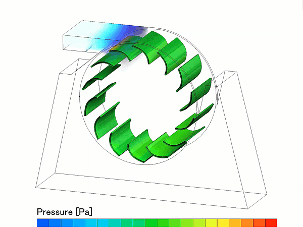
In the deployment of renewable hydrokinetic energy infrastructure—spanning tidal channels, run-of-river installations, and low-head industrial outfalls—the cross-flow water turbine (often deployed as a Darrieus or Savonius-type vertical axis hydrokinetic turbine) is a vital tool for decentralized power generation. By operating with a rotational axis oriented perpendicular to the incoming water stream, these turbines capture kinetic energy from any directional flow without requiring expensive yaw-mechanism controls.
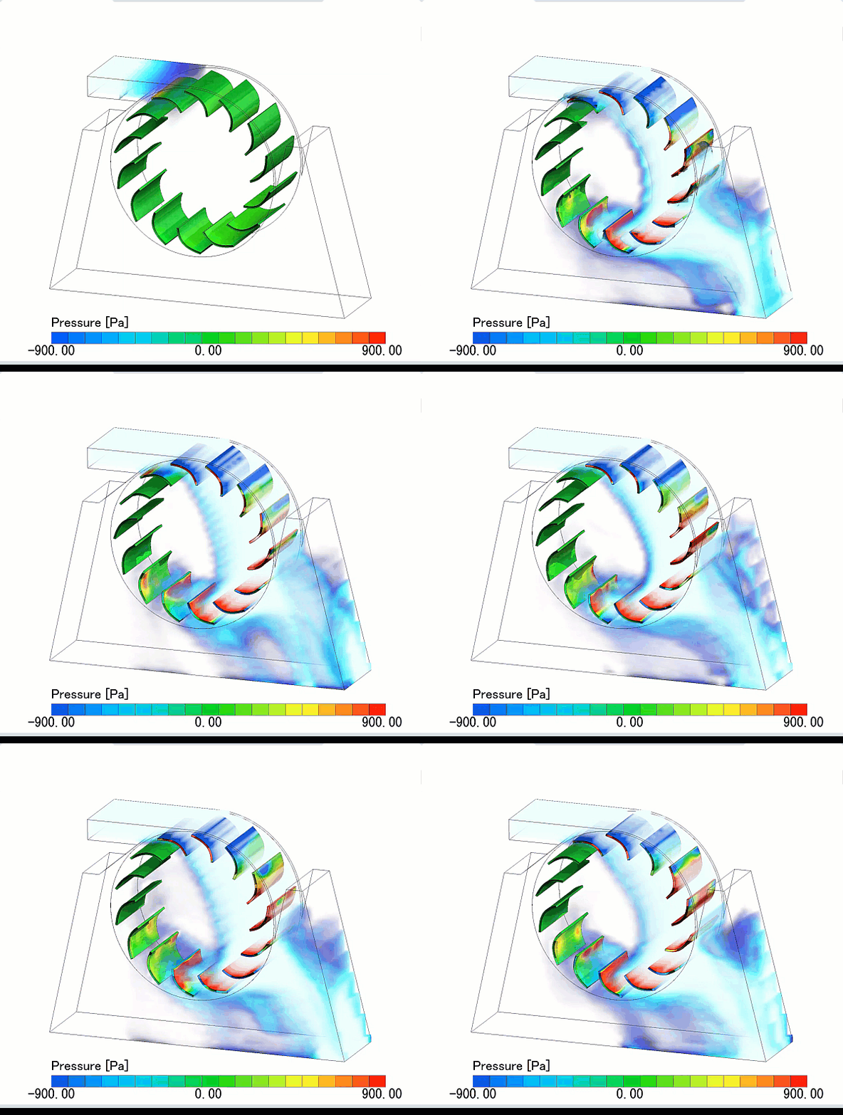
Operating a hydrokinetic turbine efficiently requires maximizing the hydrodynamic power coefficient (Cp) while strictly managing structural torque fluctuations and structural blade fatigue. Because liquid water is roughly 800 times denser than air, the physical load spikes experienced by a cross-flow turbine blade are exceptionally severe. Engineering teams rely heavily on Computational Fluid Dynamics (CFD) to optimize blade hydrofoil profiles, determine optimal solidity ratios, and predict operational lifespans.
However, simulating a cross-flow water turbine is an exceptionally deceptive, highly unsteady turbomachinery challenge. Unlike a standard axial propeller, where the blades experience a relatively steady angle of attack, a cross-flow blade undergoes violent, continuous aerodynamic variations every single rotation. If your simulation setup relies on steady-state rotational force approximations or coarse grid configurations, your solver will completely smooth over localized flow reversals—leaving your design team blind to efficiency-killing dynamic stall traps.
1. The Physics Anchor: Cyclic Angles of Attack and the Dynamic Stall Vortex
The transient fluid dynamics of a cross-flow water turbine are governed by the Navier-Stokes equations tightly coupled with a Rigid Body Rotational Framework. The primary metric dictating turbine efficiency is the Tip Speed Ratio (TSR), which defines the relationship between the blade’s rotational velocity and the oncoming free stream velocity.
As a hydrofoil blade sweeps through a single 360-degree rotation, it experiences a highly volatile physics loop:
[Blade Sweeps Upstream] ➔ [Effective Angle of Attack Skyrockets past Static Stall Limit] ➔ [Rolls Up Powerful Dynamic Stall Vortex] ➔ [Vortex Sheds off Trailing Edge] ➔ [Catastrophic Torque Collapse & Structural Vibration Spike]
- The Cyclic Angle of Attack: As the blade rotates from the upstream power stroke to the downstream return stroke, its relative velocity vector changes continuously. At lower tip speed ratios, the effective angle of attack swings violently, routinely blowing past the hydrofoil’s static stall threshold.
- The Dynamic Stall Vortex (DSV): When the angle of attack spikes rapidly past the static stall limit, the boundary layer does not detach instantly. Instead, it rolls up into a massive, concentrated rotational structure on the suction side of the blade—the Dynamic Stall Vortex. As long as the DSV remains attached to the upper surface, it generates an immense localized lift force, spiking the turbine’s torque output.
- The Shedding Collapse: Within fractions of a second, the high-momentum DSV migrates down the chord and detaches violently from the trailing edge. This shedding action causes an immediate, catastrophic lift collapse and a severe spike in hydrodynamic drag. The sudden loss of lift generates a massive mechanical torque shockwave that travels up the drive shaft, driving mechanical fatigue and forcing the downstream return stroke into a stagnant, low-efficiency wake.
2. Industry Context: Where Hydrokinetic Precision Prevents Blade Delamination
Optimizing hydrofoil cross-sections and managing structural fatigue loads through high-fidelity CFD directly dictates the commercial survival, warranty lifecycles, and grid synchronization stability of subsea energy assets:
- Tidal Energy Marine Arrays: Tidal currents reverse direction with the lunar cycle. Cross-flow turbines allow developers to build fixed subsea arrays that generate predictable power regardless of whether the tide is flooding or ebbing. Engineers use CFD to optimize multi-blade arrays, utilizing the wake of a leading turbine to actively focus and accelerate the fluid core into a downstream turbine, boosting collective farm efficiency.
- Run-of-River Floating Platforms: Small, ultra-slender cross-flow turbines are deployed on pontoon platforms in shallow rivers to power off-grid communities. Because these units operate near riverbeds and banks, engineers deploy transient multi-body CFD to ensure that the asymmetric boundary layers generated by the river bottom do not trigger unmanageable structural rolling moments that capsize the platform.
- Suppreessing Marine Cavitation Inception: At high rotational velocities, the extreme low-pressure peak generated inside the core of the dynamic stall vortex can cause the local static pressure to drop below the fluid’s vapor pressure. This triggers localized blade cavitation, where vapor bubbles form and violently implode against the composite structure, causing rapid pitting and structural blade delamination over months of deployment.
3. The Traps & Friction: Why Cross-Flow Turbine CFD Fails
Predicting the exact power coefficient curves and transient load fluctuations of a vertical-axis hydrokinetic vehicle requires avoiding severe numerical shortcuts. Defaulting to standard configurations leads to three severe traps:
Relying Blindly on the Moving Reference Frame (MRF) Shortcut
To bypass the computational cost of resolving a moving mesh, engineers frequently simulate rotational machinery using the steady-state Moving Reference Frame (MRF) or Frozen Rotor approach. While MRF is highly accurate for axial propellers spinning in a uniform stream, it is fundamentally useless for cross-flow turbines. Because the blades experience continuous, time-dependent variations in their local velocity vectors, the flow is inherently transient. An MRF shortcut completely flattens these cyclic angle-of-attack swings, failing to predict the birth, growth, and shedding of the dynamic stall vortex, outputting wildly over-optimistic efficiency charts.
Misconfiguring the Boundary Layer Grid and Wall Y+ Metrics
The exact inception point and shedding timing of the dynamic stall vortex are governed entirely by the fluid behavior within the microscopic viscous sublayer adjacent to the hydrofoil skin. If your volume mesh is too coarse near the blade surface, the mathematical solver will suffer from massive numerical diffusion, artificially averaging out the local velocity gradients. Without micro-scale prism layer grid refinement maintaining a strict Wall Y+ near 1 across the entire 3D span, the turbulence models will miscalculate the wall skin friction, causing the simulation to predict attached flow when the physical blade has long since entered a catastrophic stall.
Utilizing Standard Mesh Smoothing for High-Aspect Rotations
To simulate a rotating blade, the grid blocks inside the rotational zone must physically spin relative to the outer stationary fluid blocks. If you default to standard spring-based mesh smoothing or deformation algorithms to handle this motion, the cells along the rotational interface will quickly distort, skew, and pinch into zero or negative volume elements, crashing the solver within a few degrees of rotation. Overcoming this grid-motion limitation requires deploying advanced Sliding Mesh (Time-Dependent) techniques or Overset Mesh (Chimera grids), allowing a highly refined, boundary-conforming blade grid to slide cleanly over a static background ocean grid without any cell deformation.
4. Conquering the Rotational Hydrokinetic Interface
A beautiful, colorful velocity contour animation of a spinning hydrofoil is completely useless if your digital torque spikes and power coefficients do not correlate with physical telemetry. Validating your cross-flow water turbine CFD pipeline requires moving past steady-state shortcuts and deploying transient, sliding-mesh scale-resolving workflows, such as Detached Eddy Simulation (DES) or Unsteady RANS paired with transition-sensitive turbulence models (like the four-equation gamma-Re_theta transition SST model).
Your simulation parameters must be cross-referenced against empirical laboratory metrics—such as torque transducer logs, electrical load cell datasets, and Particle Image Velocimetry (PIV) wake maps validated on standardized hydrofoils in physical Hydrodynamic Towing Tanks or Circulating Water Channels—ensuring your moving mesh interfaces, boundary layer transitions, and transient vortex shedding profiles perfectly reflect physical hydrokinetic realities.
Author: Caesar Wiratama
Find me on Linkedin