
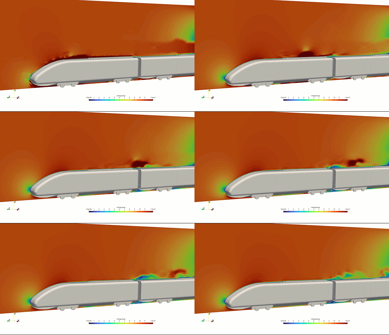
As high-speed trains breach cruising velocities of 300 kilometers per hour and beyond, mechanical resistance mechanics undergo a dramatic shift. While rolling resistance from steel-on-steel wheel contact dominates at lower speeds, aerodynamic drag scales exponentially with velocity. At modern high-speed cruise thresholds, fighting atmospheric air resistance accounts for over 80% of a train’s total energy consumption.
Unlike standard aircraft aerodynamics, where the fluid moves cleanly over a single streamlined fuselage, a train is an exceptionally long, multi-car bluff body operating in extreme proximity to a static ground plane.
Designing these next-generation locomotives via Computational Fluid Dynamics (CFD) is mandatory for manufacturers to lower traction power requirements, pass crosswind stability certification, and suppress explosive acoustic booming inside tunnels.
However, simulating high-speed train aerodynamics is a highly deceptive, transient multi-body challenge. If your digital framework relies on simplified steady-state approximations or flattens trackside boundary conditions into static walls, your solver will suffer from smeared slipstreams and output false drag peaks—leaving your design team blind to efficiency-killing flow separations and safety-critical derailment risks.
1. The Physics Anchor: Boundary Layer Accumulation and Crosswind Vorticity
The fluid dynamics surrounding a high-speed train are governed by the compressible Navier-Stokes equations tightly coupled with a highly shearing Ground Proximity Interface. The fluid path transitions through three distinct aerodynamic zones:
[Sleek Nose Impacts Air] ➔ [Massive Pressure Stagnation Peak] ➔ [Flow Runs Down Long Car Array] ➔ [Viscous Boundary Layer Accumulates & Thickens] ➔ [Unsteady Wake Separation at Tail]
- The Nose Stagnation Discontinuity: As the train’s nose punches through the air, it creates an immediate localized stagnation point where static pressure spikes violently. If this geometry is poorly contoured, it forces a massive compressed air wave forward, which translates into a devastating micro-pressure wave boom when the train enters a tunnel.
- The Boundary Layer Accumulation Trap: As the fluid flows down the length of the train (which can span over 400 meters), skin friction continuously strips momentum from the air. The viscous boundary layer thickens progressively from the nose to the tail, rolling into a turbulent, high-energy slipstream that sweeps along the sides of the cars, threatening trackside worker safety and ballast stability.
- The Tail Wake Separation: When the accumulated boundary layer reaches the trailing car, the geometry terminates. The flow detaches violently, shedding a pair of highly unsteady, counter-rotating tail vortices that create a low-pressure suction zone behind the train, cementing the net aerodynamic drag penalty.
2. Industry Context: Where Airflow Control Secures High-Speed Track Safety
Optimizing nose topologies, underbody clearance channels, and tail profiles through high-fidelity CFD directly dictates the energy footprint, routing infrastructure cost, and operational safety margins of modern rail networks:
- Tunnel Micro-Pressure Wave Mitigation: When a high-speed train enters a tunnel at 350 km/h, it acts like a piston inside a syringe, compressing the internal air into a shockwave that travels down the tunnel at the speed of sound. When this wave exits the far portal, it releases a violent acoustic boom that can damage nearby buildings. Engineers use CFD to design long, specialized bio-mimetic nose profiles (such as duck-bill or multi-sloped contours) to smooth out the initial pressure gradient.
- Crosswind Stability and Derailment Protection: High-speed trains frequently traverse exposed bridges or open plains subject to intense natural crosswinds. When a crosswind hits the train at an angle (yaw angle), the airflow separates violently along the leeward side of the leading car, creating a massive aerodynamic lift and side force. Designers deploy detailed crosswind simulations to calculate the critical wind velocity curves, ensuring the train maintains a safe weight margin against aerodynamic overturning.
- Underbody Aerodynamics and Ballast Flight: The clearance gap between the bottom of the train and the track bed houses irregular components like bogies, wheels, and brake discs. This restricted channel chokes the air, creating a high-velocity, turbulent underbody stream. This stream can suck up loose stones from the track bed (ballast flight), projecting them at high speeds against the undercarriage and causing severe mechanical damage.
3. The Traps & Friction: Why High-Speed Train CFD Fails
Predicting the exact drag profile, slipstream velocities, and side-force peaks of a multi-car rail vehicle requires navigating strict numerical and boundary traps:
Relying Solely on Steady-State RANS Solvers
To minimize massive processing times across models that stretch hundreds of meters in length, engineers frequently make the mistake of running train simulations using steady-state Reynolds-Averaged Navier-Stokes (RANS) equations. While RANS is highly efficient for baseline skin-friction calculations, it is fundamentally incapable of capturing the transient physics of wake separation and crosswind gusting. RANS artificially stabilizes the fluid fields, “smearing” the transient tail vortices into a continuous, static cloud. RANS notoriously miscalculates the base pressure at the rear car, under-predicting the actual aerodynamic drag and failing to identify peak rolling moments during crosswind gusts.
Treating the Track Bed and Wheels as Static Boundaries
A train operates inches away from a stationary track bed while its wheels spin at thousands of RPM. A common and destructive pitfall in rail CFD is treating the ground plane and wheel surfaces as static walls. If the ground boundary condition is not explicitly configured as a Moving Wall matched to the train’s forward velocity, an unphysical, sluggish boundary layer will build up underneath the locomotive on your screen. This error completely destroys the accuracy of your underbody velocity profile, rendering your ballast flight and bogie drag predictions entirely useless.
Under-Resolving the Inter-Car Gaps and Bogie Cavities
A train is not a perfectly smooth tube; it contains severe geometric discontinuities at the inter-car gangways and inside the bogie recesses. These cavities act as massive open shear layers where fluid drops into highly chaotic, recirculating eddies that sap energy from the propulsion loop. To keep cell counts low, automated meshing routines frequently coarsen the volume grid inside these gaps. This numerical smoothing under-predicts the localized pressure drag spikes, leaving your engineering team unaware that minor shielding fairings around the wheels or gangways could unlock a significant reduction in total traction power.
4. Conquering the High-Speed Ground Interface
A beautiful, colorful velocity contour plot of a streamlined locomotive profile is completely useless if your digital drag coefficients and slipstream profiles do not correlate with physical track testing. Validating your high-speed train CFD pipeline requires moving past static shortcuts and deploying fully coupled, transient scale-resolving workflows, such as Detached Eddy Simulation (DES) or Large Eddy Simulation (LES).
Your simulation parameters must be cross-referenced against empirical laboratory and field metrics—such as multi-component moving-model rig tests inside specialized Atmospheric Wind Tunnels and full-scale pitot-tube slipstream traverses conducted on real operational lines according to international standard EN 14067—ensuring your moving ground boundaries, boundary layer accumulations, and transient crosswind forces perfectly reflect physical high-speed rail realities.
Author: Caesar Wiratama
Find me on Linkedin