
Meshing or discretization is the process of dividing the continuous fluid domain into a discrete computational domain, allowing the generally nonlinear partial differential equations of fluid mechanics to be numerically solved (further details will be discussed in the solver theory chapter).
Generally, smaller mesh sizes will yield more detailed and accurate computational results but will increase the number of elements, thereby requiring higher computational efforts.
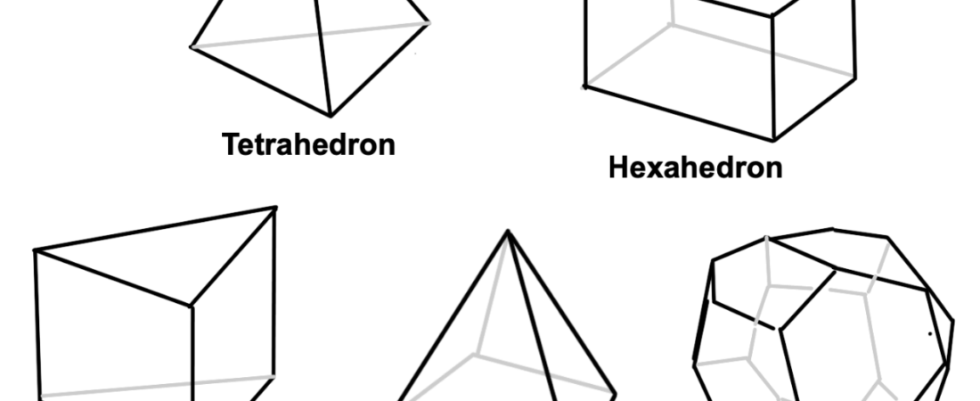
Before discuss deeper into meshing, it’s important to first understand several terminologies used in meshing, as illustrated in Figure 2.1 below:
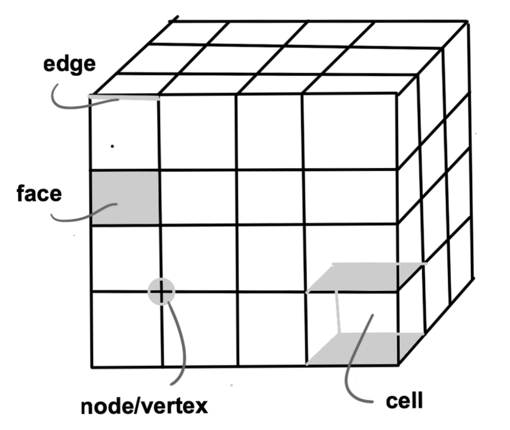
Figure 3.1. Basic Mesh Terminology
With the following definitions:
- cell – the control volume where the domain is divided
- node or vertex – the endpoint of a grid,
- cell center – the central point of a cell,
- edge – a side boundary of a face,
- face – a side boundary of a cell,
- zone – a group of nodes, faces, and cells,
- domain – a group of node, face, and cell zones.
It is important to understand the difference between mesh and geometry terminology; some software has its own terms, but generally, the “point”, “line”, and “surface” for mesh are used in the same way as “node”, “edge”, and “face” for geometry.
Some important considerations when creating a mesh include:
- Resolution or mesh detail
- Type of mesh, and
- Hardware used for the simulation (generally, higher resolution mesh needs higher RAM to store the mesh data during meshing)
3.1. Type of mesh
The shape of the control volume depends on the solver’s capabilities; structured-grid codes utilize quadrilaterals in 2D flow and hexahedrons in 3D flow.
Meanwhile, unstructured grids use triangles in 2D flow and tetrahedrons in 3D flow
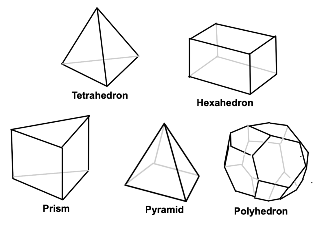
Figure 3.2. Type of mesh
In general, meshes composed of hexahedra offer advantages in terms of efficiency in the creation of element count (cells).
Imagine a 2D box requiring only one element to form a 1×1 meter square, while a triangular shape needs two elements to form the same box. This discrepancy becomes even more significant when dealing with 3D models.
Moreover, in numerical methods (to be discussed in the solver theory), data transfer is faster with a higher number of ‘neighbors’ or surfaces from these elements.
In this case, one hexahedral element has six neighbors, whereas one tetrahedral element has four neighbors, indicating that hexahedra has more neighbors.
Advancements in polyhedral mesh types aim to accommodate this advantage by increasing the number of surfaces.
Structured mesh configurations, also known as structured mesh, as illustrated in Figure 2.3, can be employed to achieve optimal data transfer. In this mesh type, data transfer speed and plotting can be performed effectively, quickly, and accurately, supporting good visualization.
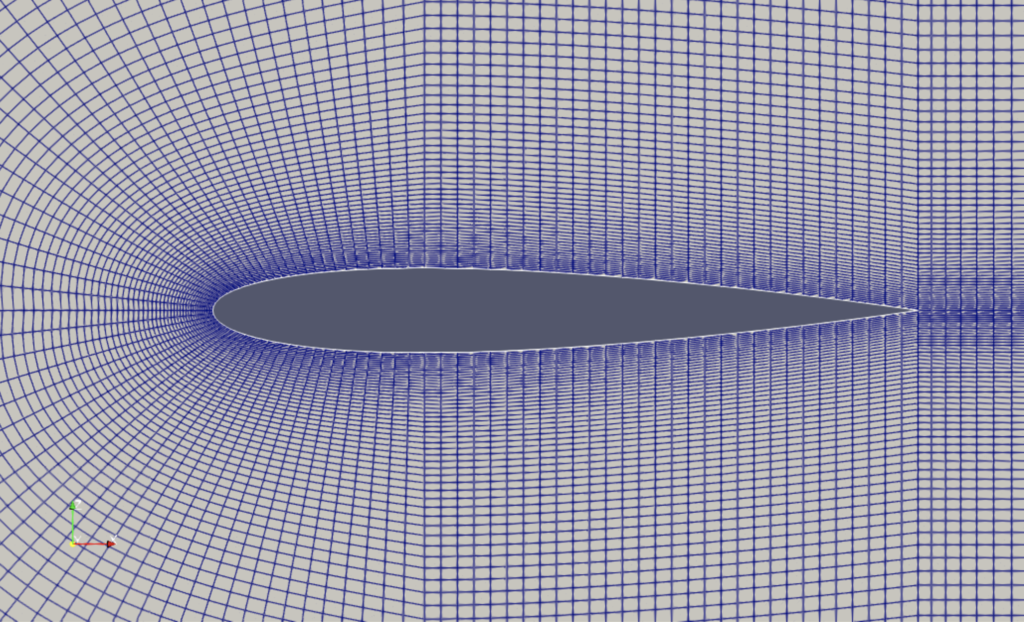
Figure 3.3. Structured grid of NACA 0012 with OpenFOAM
However, a primary drawback of hexahedral meshes is the difficulty in shaping complex geometries (although achievable, as shown in Figure 3.3, the time required to create them is not feasible for fast daily analysis).
Consequently, tetrahedral meshes have become more commonly used due to their advantage in creating complex geometries
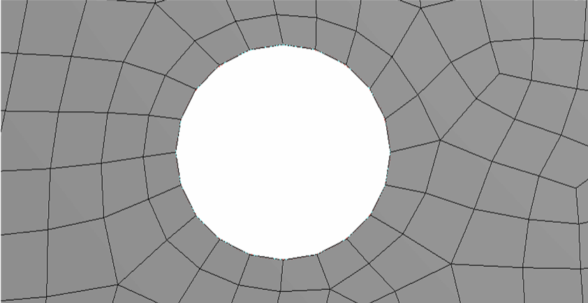
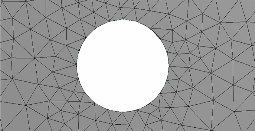
Figure 3.4. Hexa (top) versus Tetra (bottom) mesh
Besides using a single type of mesh within a domain, we can also mix different types, for instance, combining hexahedral and tetrahedral or polyhedral meshes simultaneously, known as a hybrid mesh, as illustrated in Figure 3.5.
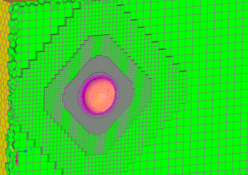
Figure 3.5. Hybrid mesh of Hexa and Polyhedron constructed with Cradle CFD
There’s also a type of mesh based on hexahedra that is quite adaptive for detailed models. This model combines a simple hexahedral block mesh ‘cut’ by the object. Then, one hexahedral block is subdivided into smaller sizes in the areas around the walls to form the required geometric details.
In software like OpenFOAM, this type of mesh is known as snappyHexMesh.
Figure 3.6 illustrates the snappyHexMesh created using openFOAM software.
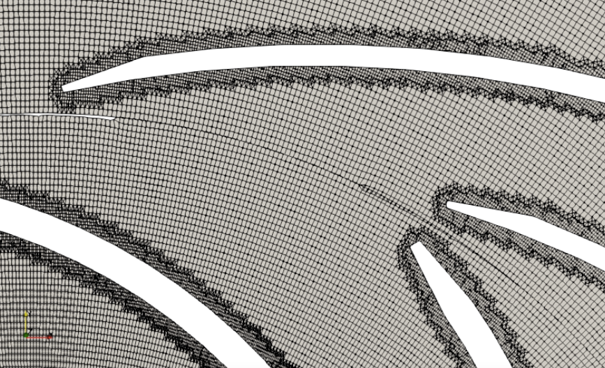
Figure 3.6. SnappyHexMesh generated with OpenFOAM
3.2. Mesh Inflation
In fluid mechanics theory, we recognize the presence of fluid flow conditions that tend to adhere to solid walls, also known as the no-slip condition.
This condition causes the velocity gradient around the surface to have specific patterns determining several parameters like shear stress, convection coefficients, and others, forming a layer with a specific thickness known as the boundary layer.
Typically, this layer is very thin, requiring a significant amount of mesh if we were to create mesh sizes around this layer equivalent to the boundary layer’s thickness.
One method to accommodate this boundary layer thickness without altering the entire mesh size in detail is inflation. It involves creating layered mesh along the normal direction to the wall surface, as illustrated in Figure 3.7.
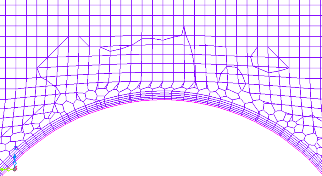
Figure 3.7. Mesh inflation layer around an object
Since this mesh only extends in the normal direction from the surface (in mathematical terms, upwards from a coordinate system, typically the Y-axis), it’s commonly referred to as the positive Y-direction or the inflation direction, or .
3.3. Wall Distance and y+ value
The calculation concept Is very useful for determining the minimum inflation layer thickness around the wall to accommodate the boundary layer.
Mathematically, defined as:
(3.1)
Where is the friction velocity around the wall, y is the closest distance to the wall, and
is the shear stress. The mathematical form above is not an equation but an equivalence, as the use of the concept
is merely an initial estimate that can have different definitions depending on the method used by the researcher because it’s a non-dimensional parameter.
The calculation is commonly performed using an online calculator by inputting the desired value, free stream velocity, Reynolds number, as well as the density and viscosity of the fluid, to obtain the initial inflation thickness in the mesh we will use.
It’s important to note that flows with high Reynolds numbers, such as those around high-speed aircraft or projectiles, will have very thin boundary layers. Therefore, the use of inflation becomes less significant and can be disregarded.
Another important aspect to note is that doesn’t always have to perfectly capture the boundary layer. In turbulent modeling, there are features called wall functions that will be specifically discussed in the turbulent modeling chapter.
Since y+ value is typically complex to estimate, you can use an online calculator such as this to estimate it quickly: https://pttensor.com/2024/09/13/compute-mesh-spacing-with-given-desired-y-value/
In that online calculator, we use simple estimation from flat-plate boundary layer approximation:
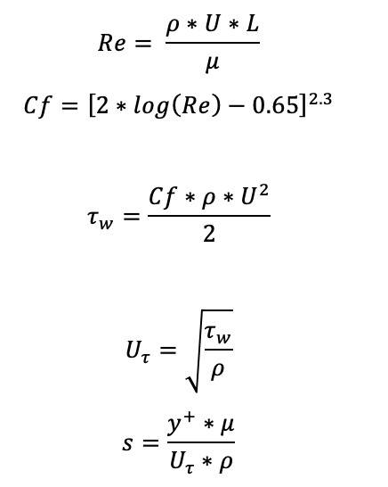
With:
Re = Reynold number
U = Free stream velocity (m/s)
Cf = Friction coefficient
s = wall spacing (m)
You can use the s value as the first layer thickness of your mesh to obtain your desired calculation accuracy and speed.
The equation for Cf is an approximation for Re < 1E+9 (From reference: Schlichting, Hermann (1979), Boundary Layer Theory, ISBN 0-07-055334-3, 7th Edition), values beyond this range must be carefully evaluated. The Cf equations are widely available with different conditions and Reynold numbers.
3.3.1. Boundary Layer Resolution:
For accurate boundary layer resolution, the grid spacing should be such that y+ falls within a specific range. This ensures that the near-wall region is resolved correctly and that the turbulence model used in the simulation operates within its valid range.
3.3.2. Typical y+ Ranges:
- Laminar Flow: In laminar boundary layers, the first cell’s y+ should ideally be very small (often y+ < 1).
- Turbulent Flow: For turbulence modeling, different turbulence models require different y+ ranges:
- Standard Wall Functions: Typically, y+ should be between 30 and 300.
- Low-Reynolds Number Models: Typically, y+ should be less than 5 to 10, with the grid sufficiently fine to resolve the viscous sub-layer.
3.3.3. Wall Functions:
- High y+: If y+ is high (e.g., greater than 30), wall functions are often used to estimate the near-wall behavior without resolving the viscous sub-layer explicitly.
- Low y+: If y+ is low (e.g., less than 5), the grid must be sufficiently fine to resolve the near-wall region accurately, and the turbulence model can be applied more directly.
3.4. Mesh Quality
The quality of the mesh is crucial to ensure simulation results align with expectations, ensuring good visualization, and in certain conditions, a low-quality mesh can cause simulations to diverge or even error in the first iteration.
Visually, we can assess the mesh quality based on its proportionality. However, this assessment is limited to the ability to judge proportionality and becomes significantly complex in evaluating detailed 3D domains. Hence, this chapter will discuss several indicators of mesh quality. Here are some commonly used mesh parameters:
3.3.1. Skewness
Skewness is used to indicate how tilted a mesh is. The more acute the angles of an element, the better the data transfer from one element to another. Hence, when the shape of an element becomes skewed, it requires significant corrections during the computation process, which reduces calculation quality and slows down computation.
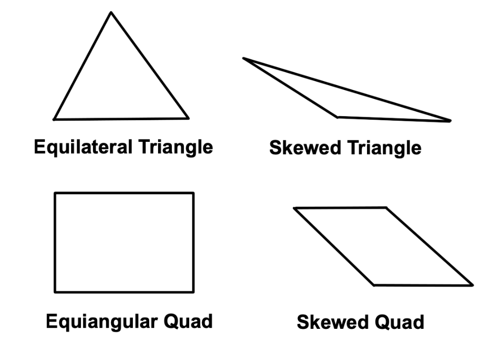
Figure 3.8. Mesh skewness
Mathematically, skewness is defined as follows:
(3.2)
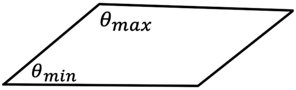
Figure 3.9. Mesh skewness calculation
With the is the equiangular face/cell (60 deg for tetra, and 90 deg for quads or hexa).
Please note that some software might have different definition of skewness, but you can understand the physical meaning from the equation (3.2) above.
Here are some general rules of thumb commonly used to assess mesh quality based on skewness (again, different software might have difference values):
Table 3.1. Mesh skewness Rule of thumb
| Skewness | Cell quality |
| 1 | Degenerate |
| 0.9 < 1 | Bad |
| 0.75 – 0.9 | Poor |
| 0.5 – 0.75 | Fair |
| 0.25 – 0.5 | Good |
| >0 – 0.25 | Excellent |
| 0 | Equilateral |
3.3.2. Aspect ratio
Aspect ratio is the comparison between the longest length of an edge and the shortest length of an edge, where a larger aspect ratio results in a slender mesh.
The ideal value for the aspect ratio is 1, signifying that the length, width, and height are exactly the same. Higher aspect ratios reduce mesh quality.
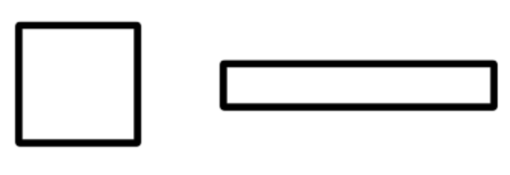
Figure 3.10. AR = 1 (left), and high AR (right)
3.3.3. Orthogonality
Orthogonality defines the orientation between one element and another, where a more parallel orientation of vectors from the center to the center of an element indicates good mesh quality as it facilitates the flow of data transfer from one element to another.
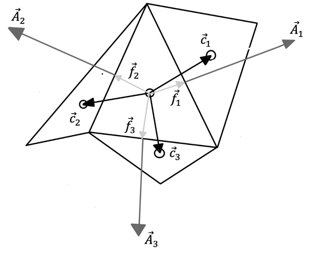
Figure 3.11. Vectors definition for orthogonality calculation
From Figure 3.11 above, orthogonality can be calculated as follows:
(3.3)
Which indicates the dot product (cosine multiplication) between the surface normal vector and the normal orientation vector from the center of element
.
Then, the orientation between the surface normal vector and the center-to-center orientation vector of the element, is also calculated, given as follows:
(3.4)
The smaller the angle difference between and
, or
and
, the closer their dot product will be to 1. Thus, equations (3.3) and (3.4) will approach a value of zero, indicating good mesh quality.
Meanwhile, the worst skewness displayed on the mesh quality monitor is the highest value calculated from equations (3.3) and (3.4).
3.4. Grid Independence Test (GIT)
The meshing process cannot be entirely calculated analytically, such as mesh size, y+ size, mesh type, and so on.
This occurs due to the nature of the geometry and physical phenomena itself, which is generally complex. For instance, it’s impractical to compute each component for the ‘perfect’ mesh in simulating a race car with specific details. There’s an element of ‘art’ and experience involved for the operator.
Nevertheless, one commonly used method to verify the suitability of the mesh is to ensure that when we slightly modify our mesh settings, it does not affect the simulation results. In other words, the simulation results become insensitive or independent of the mesh settings. This testing process is known as “mesh sensitivity test” or “grid independence test (GIT)”.
There aren’t specific rules discussing this method because each simulation has different objectives.
For example, when testing a heat exchanger with the same model, one researcher wants to analyze the pressure drop, while another wants to focus on temperature changes. Hence, their GIT parameters will differ.
For instance, the first researcher will create a test for pressure drop changes concerning grid settings, while the second will test temperature changes concerning grid settings.
The next point is defining what should be modified in the grid settings. Generally, the independent variable used is the number of elements or grids for simulations covering a large domain. For geometries with numerous walls and relatively low Reynolds numbers, variations in y+ are commonly used.
However, all choices, both for independent and dependent variables, heavily depend on the specific case at hand.
In the example below, GIT is conducted on a NACA 2412 airfoil CFD simulation using openFOAM software. In this scenario, the researcher aims to find the most suitable mesh refinement settings around the airfoil, where higher refinement leads to more cells.
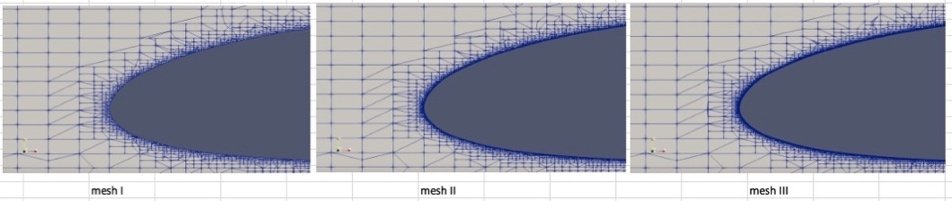
Figure 3.12. Comparison of mesh with different refinements
Therefore, in this scenario, a graph of the lift generated by the airfoil against the number of cells was created. Here are the results:
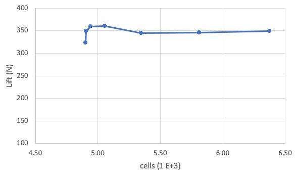
Figure 3.13. Lift versus number of cells of an airfoil CFD simulation
From the above graph, it can be shown that with the number of cells exceeding 5,000, the lift force tends to remain constant with an increase in the number of cells.
We can conclude that using a mesh with 5,500 cells will yield the same lift force as a mesh with 6,500 or more cells, requiring significantly more computational effort than the 5,500-cell mesh.
Based on these results, we can select the most optimal mesh to be used, which is the 5,500-cell mesh. However, this conclusion only applies to lift force calculations. For computations involving frictional forces, vortexes, and others, this may not hold true and should be tested based on the specific case.
3.5. Adaptive and Dynamic mesh modeling
In some specific cases, we might not be able to use a constant-sized mesh model. For instance, when simulating air inside an inflated balloon, the outer mesh size, namely the balloon’s diameter, will increase due to fluid pressure.
In more technical cases, such as the up-and-down movement of a piston in a cylinder or the opening and closing of a valve, we are required to use a changing mesh, known as a dynamic mesh.
The local adaptive mesh is sometimes also required to refine some specific areas of mesh based on the fluid motion. For example, refinement of a zone near the spray nozzle or free surface to save the computational effort.
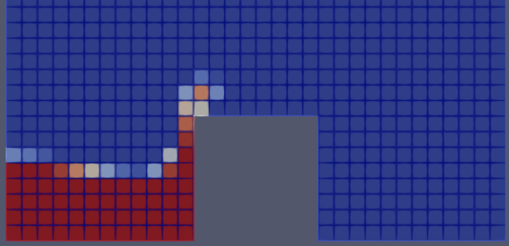
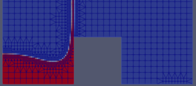
Figure 3.14. Multiphase Unrefined (top) vs Local refined mesh (bottom) in OpenFOAM
For cases involving movements characterized by uniformity in a specific orientation, such as the rotor of a centrifugal blower, it can be modeled by using more than one region connected with a interface.
A surface that moves relatively between the outer and inner parts is required to connect data from the inside and outside sections. This is also known as a sliding interface, as illustrated in Figure 2.15.
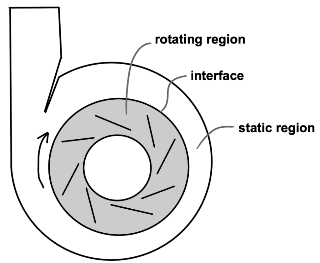
Figure 3.15. Sliding mesh
Due to the relative sliding motion between the outer and inner meshes, this modeling is also known as a sliding mesh. Sliding meshes can be created for both rotational and translational motions.
The input for dynamic mesh motion can be defined as constraints, for instance, linear movement forwards and backward, as seen in valve cases, or it could be a constant rotational speed input, such as in the case of a centrifugal blower.
3.6. Overset Mesh
Another meshing technique to simplify the simulation is using Overset Mesh, which is cell-to-cell mappings between multiple disconnected mesh regions.
This allows complex mesh geometry and motion without deforming the mesh discussed in the previous chapter; deforming mesh is often very prone to mesh quality problems, which leads to divergence.
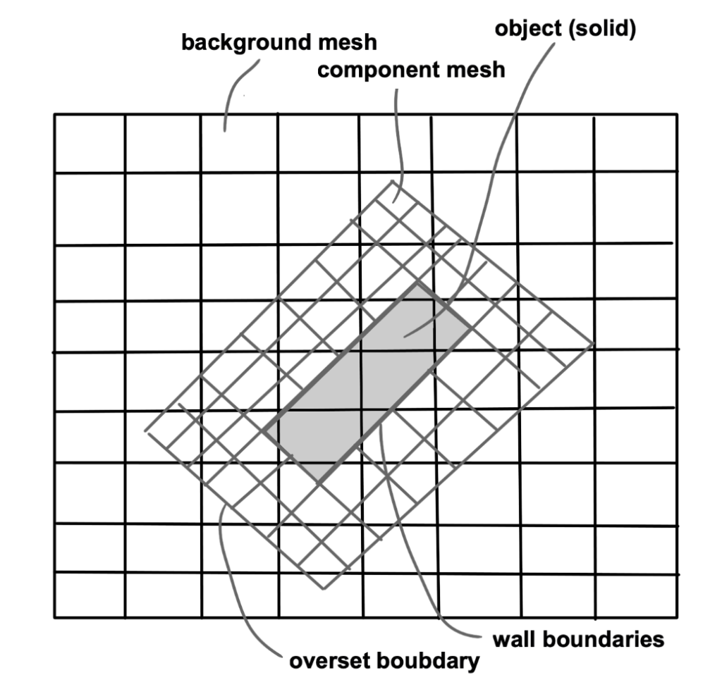
Figure 3.16. Overset Mesh
Both dynamic and overset Mesh are possible to perform a 6-degree of freedom (6 DOF) modeling. This involves dynamic mesh movement that depends on the forces generated on the surface. For instance, a turbine subjected to a flow will rotate at a specific speed as its output.
Additionally, we can consider the effects of inertia (both mass and rotational inertia moments) to observe the dynamic response of an object. For example, the motion of a ship’s hull in response to water waves.
Figure 2.17 shows an example of floating box motion on a free surface using 6 DOF overset mesh modeling.
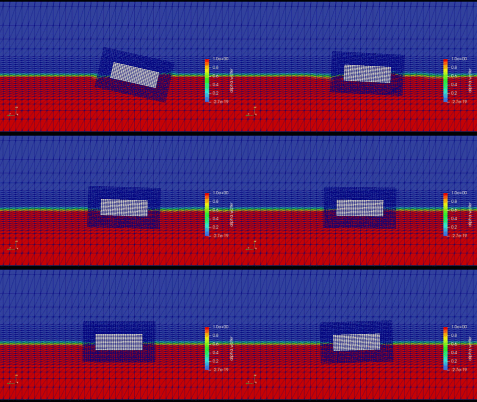
Figure 3.17. Floating body motion using an overset mesh with OpenFOAM
Author: Caesar Wiratama
Find me on Linkedin