
The fluid mechanics equation defined by the law of conservation of momentum, such as the Bernoulli equation, requires a flow that consists only of a single streamline to be solvable.
Consequently, the more general Navier-Stokes equation can more comprehensively model fluid flow within specific velocity or pressure fields. However, it’s important to note that the form of the Navier-Stokes equation is a non-linear partial differential equation, which, even as of the writing of this book, cannot be solved analytically and has smooth solutions under all conditions.
The difficulty in analytically modeling fluid flow equations arises from the existence of highly random and unsteady flow conditions known as turbulence.
Rather than attempting analytic solutions, researchers and engineers often simplify turbulent flow using specific modeling frameworks, known as turbulence modeling, enabling solutions through computer simulations (using CFD) without needing to compute detailed velocity and pressure fields.
Following is the general figure of turbulence modeling:
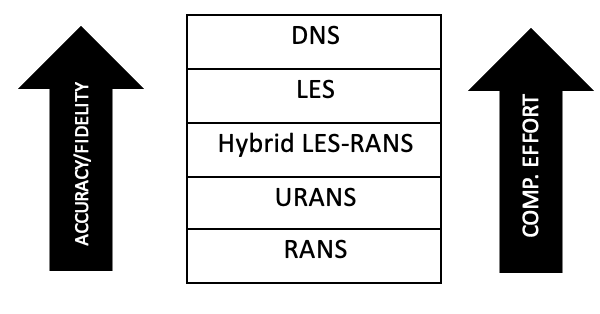
Figure 7.1. General Figure of Turbulence Models
The general rule is the higher the fidelity or accuracy of the model, the higher the computational effort. While methods like Direct Numerical Simulation (DNS) directly solve turbulent flows and can produce highly realistic and detailed solutions, DNS modeling is rarely encountered in general CFD programs due to the exceedingly high computational effort required, making it infeasible for everyday needs.
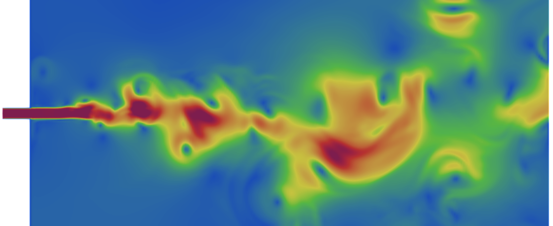
The Figure below shows the velocity distribution of a jet flow resulting from RANS and LES simulation. To capture the instantaneous velocity of a transient flow, RANS clearly doesn’t capture the detailed flow pattern compared to LES. But, the computational effort needed by the LES simulation is relatively higher. Although some LES modeling has been developed to reduce the effort, RANS is still more feasible for “daily-life” problems.
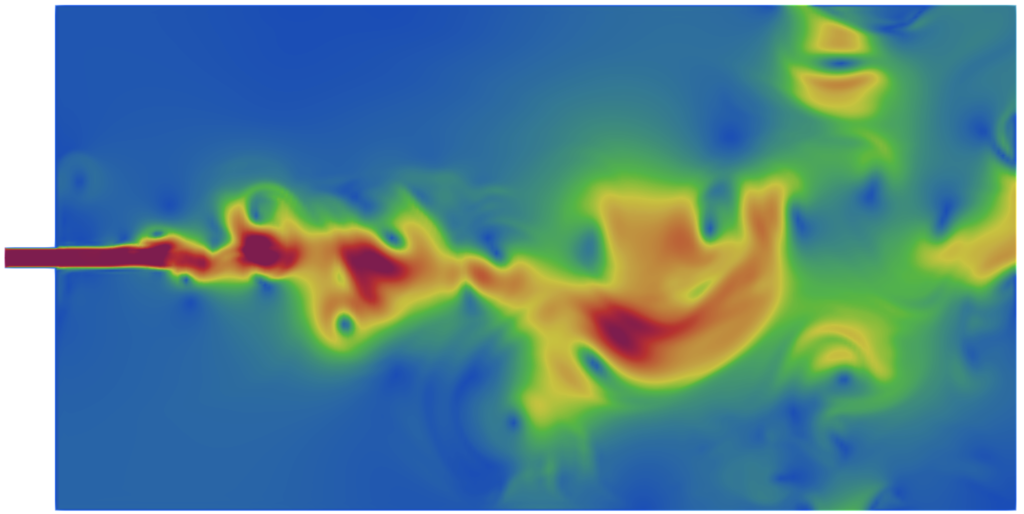
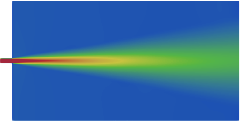
Figure 7.2. LES (top) vs RANS (bottom) instantaneus velocity result
7.1. Basic of turbulence
Turbulence modeling remains a continuously evolving discipline even today due to the highly fluctuating and complex nature of fluid flow conditions.
One of the complexities in studying turbulence is the scale or size range, which spans a wide spectrum, ranging from scales close to particle sizes to enormously large scales (kilometers) for flows in the Earth’s atmosphere or cosmic dust streams.
The diagram below illustrates the length scales of turbulent flows:
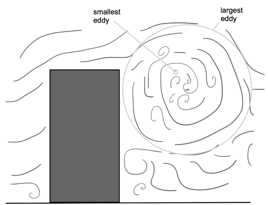
Figure 7.3. Turbulent eddies scale illustration
Let’s say we have a 100-meter building. The largest eddy size will be about a dozen meters, and the smallest are just in the order of millimeters, not to mention the eddy size near the walls.
This extreme size discrepancy makes equations (or mesh sizes) too expensive to capture all these phenomena if demanded.
The difference eddy diameter size also indicates the different characteristic of time-scale. Smaller the eddy, the “frequency” of fluid moving become larger. Which inturn makes the timestep needs to be extremily small to fully resolve it.
To date, there isn’t an exact definition of turbulent flow, but several characteristics define turbulent flow:
- Irregularity: Turbulent flow is highly irregular and chaotic, making it extremely difficult to calculate directly using the Navier-Stokes equations. Within this flow, localized vortices or eddies of varying sizes occur.
- Diffusivity: Flow containing these eddies results in internal frictions, increasing momentum exchange, such as within the boundary layer. This increased diffusivity also elevates wall drag forces and convective heat transfer near walls.
- High Reynolds Number: Turbulent flows generally occur at relatively high Reynolds numbers. For instance, in pipes, the transition from laminar to turbulent flow occurs at Re 2,300, and in the boundary layer at Re 500,000.
- Three dimensions: Turbulent flow always exists in a 3D domain due to eddies flowing in all directions, and it’s unsteady. In turbulence modeling, averaging over time and considering 2D simplifies calculations.
- Dissipation: Dissipative flow involves the conversion of kinetic energy within the flow into thermal energy (heat). This energy change occurs at small eddy scales. Small eddies gain energy from slightly larger eddies, continuing in a cascade until reaching the largest scale, while the largest eddies receive energy from the average flow. The process of transferring energy from the largest to the smallest eddies is known as the cascade process.
- Continuum: Despite eddies being very small in size, they remain significantly larger than the size of fluid molecules. Hence, mathematically, we still calculate this flow as a continuum.
Due to these characteristics, solving the Navier-Stokes equations for every detail of the flow is nearly impossible. Therefore, the simplest approach is to model it as simpler quantities and solve to obtain the required flow patterns, known as turbulent modeling.
This chapter will explain several commonly used methods in CFD for this purpose.
7.2. Reynolds (Ensemble) Averaging
In Reynolds averaging, variables from the solution of the Navier-Stokes equations are decomposed into (1) ensemble averaging or time averaging and (2) fluctuating components, as illustrated in the diagram below for velocity.
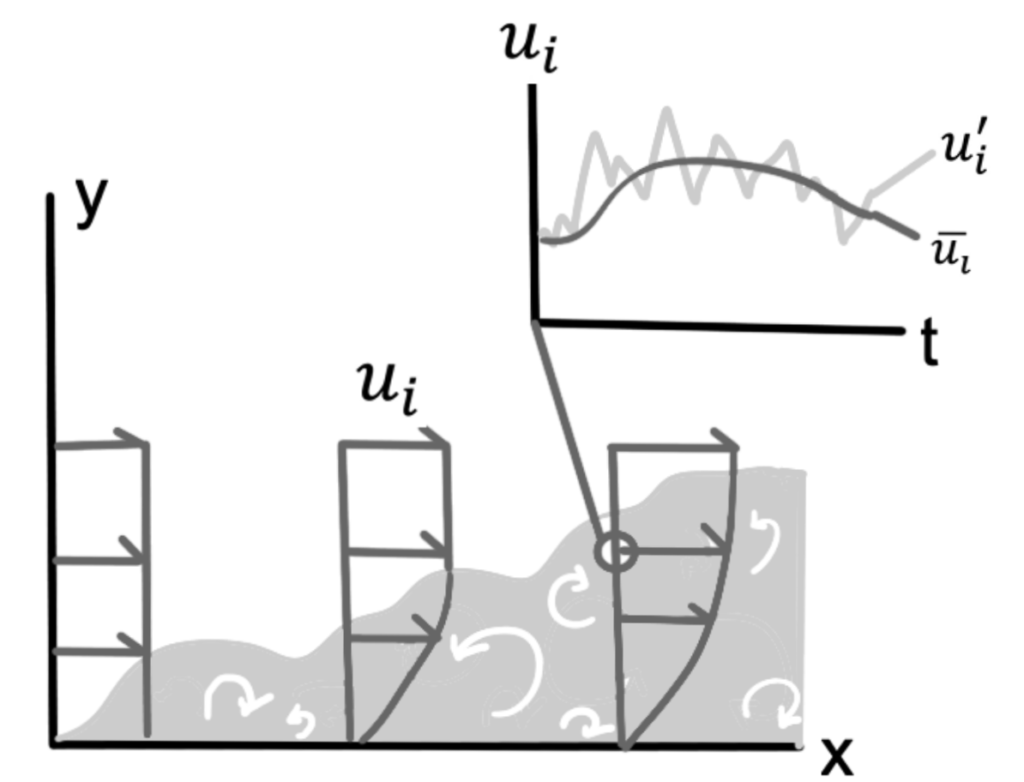
Figure 7.4. Averaged fluctuative velocity
For example, for velocity, it can be expressed as the following equation:
(7.1)
Where represents the average component, and
represents the fluctuating component (i = 1,2,3).
Similarly, for scalar quantities like pressure, energy, or species concentration, denoted as , the equation can be written as follows:
(7.2)
Substitute equations (6.1) and (6.2) into the momentum and continuity equations at an instantaneous level, then average them over time. This yields equations that can be expressed in Cartesian tensor form as follows:
(7.3)
And, for momentum equation:
(7.4)
Equations (6.3) and (6.4) are referred to as the Reynolds-averaged Navier-Stokes (RANS) equations. Additionally, the form of the term is also known as Reynolds stresses.
7.3. Boussinesq vs Reynold Stress Transport
In the previous modeling, the momentum equation includes the term Reynolds stress, which is modeled. One commonly used modeling approach is the Boussinesq hypothesis, which connects Reynolds stress with velocity gradients:
(7.5)
The Boussinesq hypothesis is used in the Spalart-Allmaras, κ-ε, and κ-ω models.
One advantage of this approach is its low computational effort, especially in calculating turbulent viscosity, , which only requires solving an additional transport equation.
From the explanation above, κ, ε, and ω respectively represent turbulence kinetic energy, turbulent dissipation rate, and specific dissipation rate.
However, the Boussinesq approach has a drawback in assuming as a scalar isotropic, which sometimes isn’t entirely accurate but remains sufficiently accurate for flows dominated by shear, such as boundary layers, mixing layers, jets, and others.
Another approach is Reynolds Stress Transport (RSM), which solves transport equations for the Reynolds stress tensor, requiring five to seven additional transport equations.
The RSM model is superior to Boussinesq for flows dominated by turbulent anisotropy, such as swirling flows or stress-driven secondary flows.
Author: Caesar Wiratama
Find me on Linkedin