
Unlike solid mechanics, fluid mechanics theories have been quite challenging to solve analytically for centuries. Hence, the easiest way to analyze and make engineering innovations related to fluid flow phenomena has been through experiments.
However, with the advancement of computational technology, it became possible for humans to solve highly complex discrete equations using computers within a reasonable time. Computational Fluid Dynamics, or CFD, is the computational method used to solve these discrete fluid equations.
As it has evolved, CFD methods have become capable of handling various fluid flow cases, ranging from incompressible flows like those around race cars to compressible flows like those around supersonic jets to complex flows involving combustion, multiphase flows, particle interactions, and more.
This book will discuss CFD from basic computation and modeling techniques. But first, the “FD” of CFD is “Fluid Dynamics,” so we must first discuss about the fluid dynamics or at least define some basic understanding of it.
To model fluid flows, similar to classical physics theories in general, three governing equations define the conservation laws: the conservation of mass (continuity), the conservation of momentum (Navier-Stokes equations), and the conservation of energy.
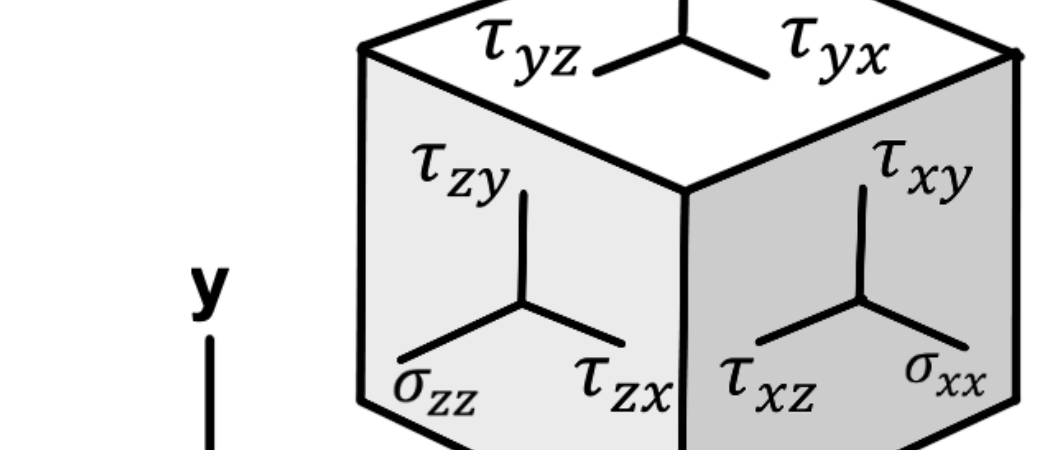
Some properties like velocity, pressure, shear stress, and temperature are typically used to define the fluid flow phenomena which are constructed in the governing equations.
- Fluid Flow ParametersPressure
Pressure is defined as the force divided by the area perpendicular to the normal direction.
(2.1)
With , and p are force vector, unit normal vector, surface area, and pressure, respectively.
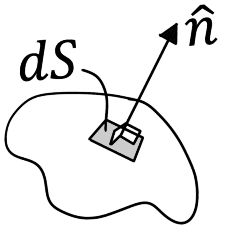
Figure 2.1. Normal vector of a surface
By definition (in physics), this is the same as normal stress, but in engineering, we use pressure as the exerted load on a surface, while stress is the amount of force per area experienced by a material.
In a CFD solver like OpenFOAM, the pressure is often divided by the density to simplify the calculation.
- Velocity
Like pressure, one of the major parameters to solve in fluid dynamics is velocity, which is the vector quantity defined by the rate of change of a particle’s position with respect to time.
(2.2)
And in the vector form can be defined as:
(2.3)
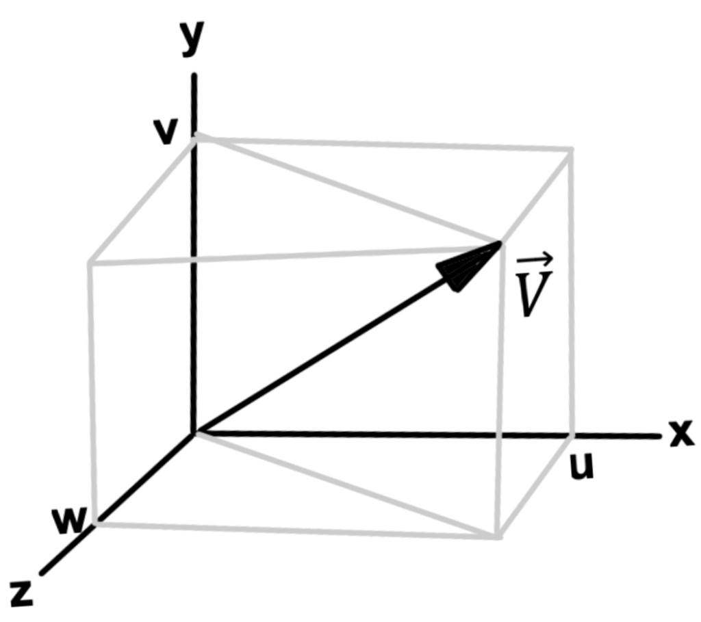
Figure 2.2. Velocity vector
- Viscosity
The major force acting on a fluid besides the pressure is the shear force, , which is defined by the properties of the fluid called viscosity defined with Newton’s law of viscosity; for Newtonian flow:
(2.4)
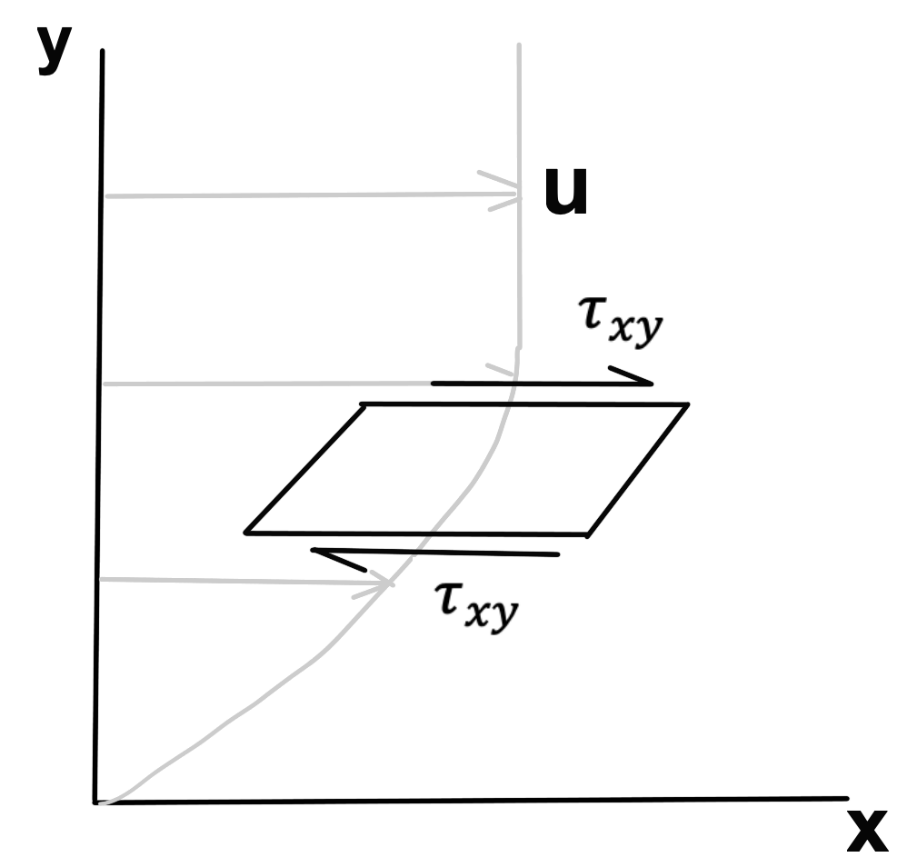
Figure 2.3. Shear stress
With is the kinematic viscosity of the fluid. The equation defines that shear force is proportional to the velocity gradient, has nine components (xx, yy, xx, xy, xz, etc.), and is often stated in the tensor form.
(2.5)
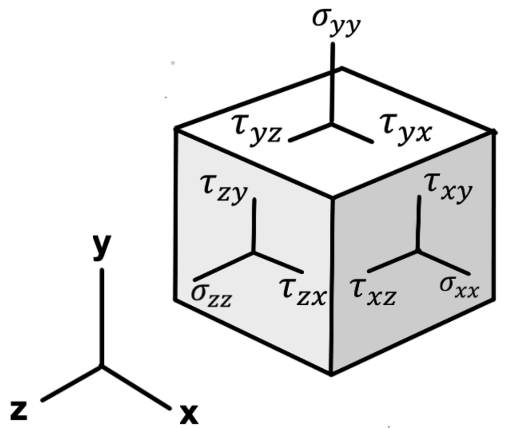
Figure 2.4. Stress tensor
- Temperature and heat transfers
Three major heat transfer methods are conduction, convection, and radiation, can be simulated using CFD simulation, which we will discuss in detail in the “heat transfer” chapter.
Following are the heat transfer equations:
- Conduction (Fourier’s law):
(2.6)
With T, , k,
, and
are temperature, heat generation per unit volume, material conductivity, and specific heat respectively.
- Convection (Newton’s law of cooling):
(2.7)
With h is (convection) heat transfer coefficient.
- Radiation (stefan-Boltzmann’s law):
(2.8)
With and
are surface emissivity and Stefan-Boltzmann constant (5.67*10-8 W.m-2.K-4), respectively.
- Fluid mechanics governing equations
Some books define the three governing equations of fluids as the Navier-Stokes equations. However, it generally defined that the Navier-Stokes equations only represent the momentum equation. We will use the “NS equation” in the rest of this book as momentum equation.
Below are explanations for each of the governing equations of fluid mechanics:
- Mass Conservation equation (continuity)
The continuity equation can be defined as follows:
(2.9)
Equation (1.9) above is the general law of mass conservation equation that applies to compressible and incompressible flows.
Where is the source term for added mass. For example, in modeling the dispersion of the second phase (e.g., evaporation) or a source defined as desired.
- Momentum conservation equation (Navier-Stokes)
The Navier-Stokes equation has some forms; this is one of the “popular” Navier-Stokes equation:
(1.10)
With is the stress tensor, p,
and
respectively, refers to pressure, gravitational load (from within the fluid itself), and external forces such as interactions with other dispersed phases or porous media.
The stress tensor itself is defined as follows:
(2.11)
With is molecular viscosity, and
is a unit tensor.
- Energy equation
The conservation of energy equation in fluid flow is defined as follows:
(2.12)
With E, h, and J respectively are total energy, enthalpy, and mass flux.
Compressible Flow
For high-speed gas fluid flow (more than 0.3 speed of sound), the gas density, which is assumed to be constant in some simple modeling, can change due to significant pressure variations.
The speed of sound is characterized by the Mach number, M, defined as follows:
(2.13)
Where c is the speed of sound in the gas, which can be calculated using the equation:
(2.14)
With is the gas specific heat ratio (CP/CV).
In CFD modeling, you only need to activate the non-constant fluid density, for instance, using the ideal gas equation or real gas equation to consider the compressible flow.
But, changing the non-constant density can make your solver sensitive to divergence because it involves temperature and pressure changes, making the solution much more complex.
The selection between pressure-based and density-based solvers will be discussed in the solver theory chapter, but essentially, compressible flows can be solved by both pressure-based and density-based solvers.
We must pay special attention to the compressible boundary conditions, which will be discussed in the chapter on boundary conditions.
Inviscid flow
In real-world applications, there’s no fluid completely free from the effects of viscosity. However, the transition from inviscid to viscous modeling in numerical CFD modeling entails significantly different computational efforts. Inviscid models are mathematically straightforward, resulting in much faster computational times.
Cases that can be modeled using inviscid approaches involve very high Reynolds numbers, where the inertia effects in the flow dominate significantly over external forces (friction) indicated by a very thin boundary layer (BL). Examples include flow-around projectiles or high-speed aircraft.
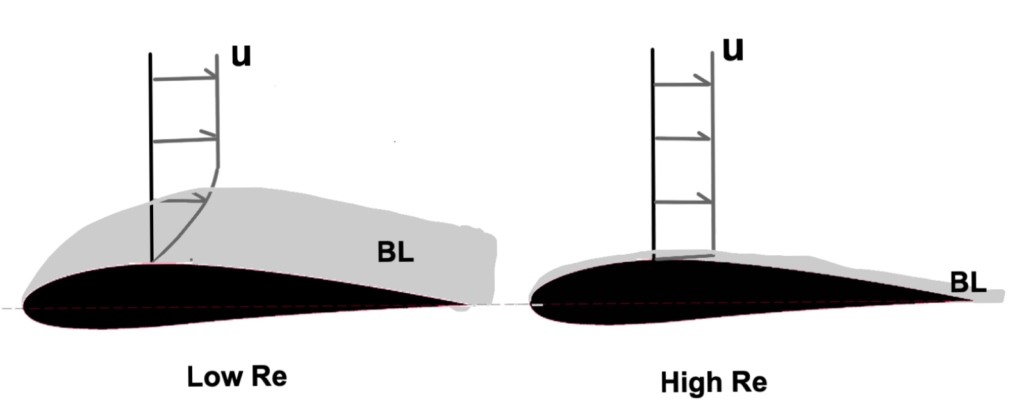
Figure 2.5. Low vs High Reynold Number Boundary Layer (Exagerated)
While unable to accurately predict lift and drag, inviscid modeling allows for quick trend analysis to find the most optimal designs. After obtaining such designs, one can analyze them using viscous models to gather detailed data.
The mathematical form of the inviscid equations for continuity is the same as equation 2.9. Then, the momentum equation is equation (1.10) with = 0, while the conservation of energy equation is defined as follows:
(2.15)
With is the source term for energy. The governing equations for inviscid flow mentioned above are also known as the Euler equations.
Author: Caesar Wiratama
Find me on Linkedin