
The idea of Computational Fluid Dynamics (CFD) modeling and simulation is solving the integral-differential equations from the Navier-Stokes equations or other transport equations using numerical algebraic equations.
However, modeling these equations is not always straightforward due to their complexity or the interconnection of numerous parameters. Therefore, several algorithms have been developed to solve them, and we’ll discuss them one by one in this chapter.
To avoid complexity, this chapter will not discuss the detailed matrix equations in-depth, but it will focus on some best practices to be used as your reference or at least “educated guess” for your setups.
5.1. Navier Stokes Equation terms
As explained in Chapter 1, with equation (1.10), the Navier-Stokes equation (or momentum equation) consists of a non-linear partial differential equation, which is the sum of some terms that have different methods to solve analytically or numerically.
Hence, it is important to understand each term of this equation before further discussing the numerical scheme.
Let’s rewrite the equation (1.10) here:
(5.1)
= transient term
= convective term
= pressure (gradient) term
= stress term, which is often reduced to internal (viscosity) force or velocity diffusion term =
= body force (external) force term
= other external force term
5.2. Density-based and pressure-based solvers
Historically, the pressure-based approach was developed for incompressible flows at low speeds, while the density-based approach was for high-speed compressible flows. Over time, both methods have been applicable to a wide range of flow regimes.
In both approaches, velocity is obtained from the momentum equation. For density-based methods, the continuity equation is used to solve the density field, while the pressure field is computed from the equation of state.
On the other hand, in the pressure-based approach, the pressure field is obtained by solving the continuity and momentum equations.
There are two approaches within the pressure-based method: segregated, where the momentum equations are solved for each coordinate direction separately, and coupled, where all coordinates are solved simultaneously. Compared to segregated methods, the coupled approach provides faster solutions but requires 1.5 to 2 times more memory.
5.3. Scalar transport general equation
CFD modeling is typically formulated using control-volume techniques to transform general scalar transport equations into algebraic equations that can be solved numerically.
In general, a scalar quantity, let’s say , can be expressed in integral form as follows:
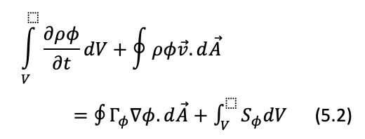
With V as the control volume, A as the area, as the diffusion coefficient, and
as the source term per unit volume, this can be discretized into the following equation:
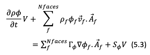
In fluid mechanics, the scalar quantity, , can be set as needed, such as for momentum, energy, turbulence, and so on.
5.4. Discretization Schemes
Several terms exist in the transport equation discussed in the previous chapter, including spatial, temporal, and gradient terms, each solved in different ways.
5.4.1. Interpolation Schemes
The interpolation schemes typically interpolate the values from cell centers to face centers. Typical interpolation schemes are summarized as follows:
Table 5.1. Interpolation scheme summary
| Scheme | Description |
| linear | Interpolation using linear equation |
| Cubic | Interpolation using cubic equation |
| Upwind | The estimation “direction” is in the direction of the flow, which is beneficial for solving an advective equation. |
| MUSCL (van leer) | High accuracy even for shocks, discontinuities, or large gradients. |
The rule of thumb is that the higher the accuracy, the lower the stability.
5.4.2. Spatial and Gradient Discretization
In solving the transport equation, it’s sometimes easier to calculate the gradient of for that quantity before solving the quantity itself, making the choice of gradient discretization crucial.
Generally, there are three discretization methods: (1) Green-Gauss cell-based, (2) Green-Gauss node-based, and (3) Least Squares cell-based. Node-based methods are typically more accurate than cell-based ones on unstructured meshes but demand more computational effort.
On the other hand, the accuracy of the least squares method is comparable to the node-based approach but requires less computational effort, making it a commonly used default in CFD solvers.
5.4.3. Divergence Schemes
The typical convection term in the N.S equation, , has a divergence equation form which generally solved with Gauss scheme with some interpolation selections as follows:
Table 5.2. Interpolation scheme for Gauss scheme
| Scheme | Behavior |
| Linear | 2nd order, unbonded |
| Skew linear | 2nd order, unbonded (more) |
| Cobic corrected | 4th order, unbonded |
| Upwind | 1st order, bounded |
| Linear upwind | 1st/2nd order, bounded |
| QUICK | 1st/2nd order, bounded |
| TVD | 1st/2nd order, bounded |
| SFCD | 2nd order, bounded |
| NVD | 1st/2nd order, bounded |
In math, bounded means “defined” within a minimum or maximum x value set.
5.4.4. First-Order and Second-Order Accuracy
For cases involving flow with mesh aligned to the flow direction, such as flow in a straight rectangular duct with a hexahedral mesh, the use of first-order discretization is sufficient.
However, for more complex flows where the flow direction doesn’t align with the mesh or with unstructured meshes, using first-order convective discretization may lead to errors due to numerical diffusion.
Therefore, for flows not aligned with the mesh or with unstructured meshes, employing second-order discretization is the better choice, even though first-order discretization converges more easily (it’s more stable).
Sometimes, it’s possible to start calculations with first-order and switch to second-order after a few iterations to stabilize solutions in cases where the flow tends to diverge.
5.4.5. Other spatial discretization methods
Several other discretization schemes, such as QUICK or third-order MUSCL, can provide better accuracy than second-order schemes in rotating and swirling flows.
There are also power law schemes that generally have similar accuracy to first-order schemes.
5.4.6. Pressure discretization schemes
For pressure variables, the use of the ‘standard’ scheme is generally sufficient, but there are some other options available:
- Body-force-weighted: for flows with significant forces acting on objects.
- PRESTO!: for high-swirl flows, high Rayleigh-number natural convection, rotating flows, flows through porous media, or extreme curvature flows.
- For compressible flows, it’s recommended to use a second-order scheme.
5.4.7. Density Discretization Schemes
Several schemes apply specifically to pressure-based compressible single-phase flow:
- First-order upwind: stable and yields reasonably good solutions for almost all flow regimes.
- For compressible flows with shock, it’s recommended to use second-order upwind or QUICK schemes.
5.4.8. Under-relaxation factors
In numerical methods, including the finite volume method used in CFD solvers, the algorithm ‘guesses’ the value of a variable in the next iteration until that variable undergoes no significant change with increasing iterations (convergence condition).
However, the guessed value provided by the solver algorithm is often too far from the expected value, which ultimately leads the solution further away, causing the values to fluctuate and even diverge from a specific value.
Hence, a parameter is needed to limit the magnitude of the variable change, for instance, change per iteration, denoted as n and also known as the under-relaxation factor (URF) or
, mathematically defined as follows
(5.4)
The value of URF ranges from 0 to 1; the higher the value, the more aggressive it becomes (faster to final value) but also prone to divergence, while smaller values offer more stability but require more iterations to converge.
5.5. Pressure-Velocity Coupling Solvers
The Navier-Stokes equation strongly couples the velocity and pressure, which make this equation challenging to be solved analytically. This is where the numerical method plays a role.
To solve the coupled parameters of pressure and velocity, several commonly used methods exist, including SIMPLE, SIMPLEC, PISO, and couple.
The SIMPLE (Semi-Implicit Method for Pressure-Linked Equations) algorithm is the most popular scheme to solve the steady-state solution.
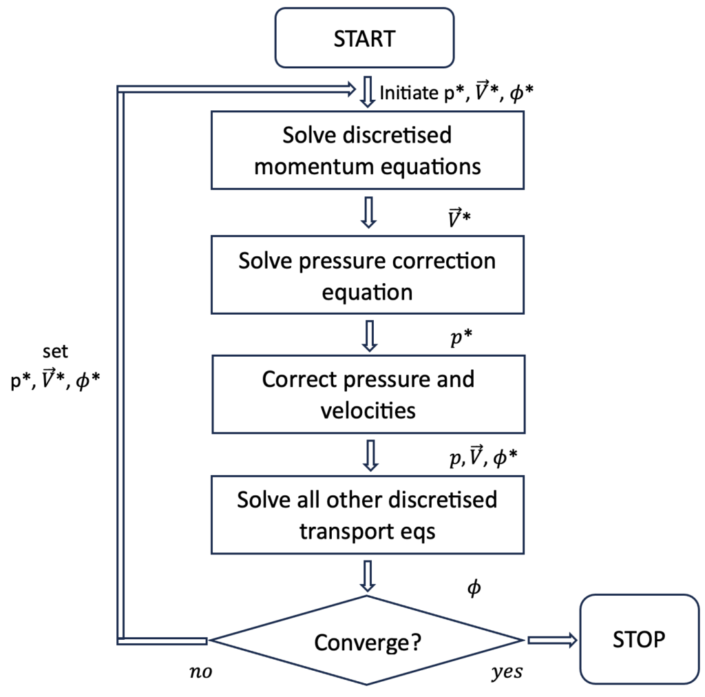
Figure 5.1. Flow chart of the SIMPLE algorithm
With * indicates the “guessing” variables.
From the illustration above, we can visualize how the velocity and pressure values are obtained in the SIMPLE algorithm, which involves guessing and an iterative process.
A transient simulation could follow the same sequence as the SIMPLE algorithm, but iterating over that sequence within each time step is costly. A more efficient algorithm solves the sequence only once per time step but adds an iterative loop that substitutes cap V ⃗ from the momentum corrector into the a term of the pressure equation, then solves the pressure equation for the second time followed by a second momentum corrector.
The addition of this “PISO (Pressure Implicit with Splitting of Operators) loop” improves the velocity calculation for the next time iteration, which increases the accuracy of the (transient) term.
SIMPLE and PISO algorithms can also be combined into PIMPLE (PISO-SIMPLE) algorithms which configured to produce a steady flow solution quickly by a pseudo-transient simulation. These simulations are not intended to capture realistic transient behavior, so they can run at a higher Courant number (Co > 1), with some under-relaxation if necessary.
For other algorithms, they won’t be extensively discussed in this book. Instead, we’ll explore the strengths and weaknesses of these algorithms as follows:
- SIMPLE: Semi-Implicit Method for Pressure Linked Equations is the most commonly used method for almost all flow regimes, especially in steady-state conditions, making it widely used as the default CFD solver.
- SIMPLEC: SIMPLE-Consistent, commonly used for simple flows, focusing only on pressure-velocity coupling, resulting in a rapid convergence of solutions.
- PISO: Pressure-Implicit with Splitting of Operators or PISO is suitable and recommended for transient simulations with relatively large time steps, but for smaller time steps such as in LES, reverting to SIMPLE or SIMPLEC might be preferred.
- Couple: This solver is quite robust and efficient, recommended for single-phase steady-state simulations.
5.6. Standard and Hybrid Initiation
Before commencing the iteration process, the equation solver algorithm requires an initial ‘guess’ to serve as the starting reference for the iterative process.
The closer this initial reference is to the expected solution, the more stable the iteration process becomes, and convergence conditions are achieved more rapidly.
For instance, imagine a straight pipe with an inlet velocity of 1 m/s. Intuitively, during convergence, the velocities across the entire pipe domain wouldn’t stray far from the value of 1. For instance, it might be 1.2 at the midsection, gradually decreasing towards the walls, yet averaging around 1.
Hence, initialization across the entire domain with the inlet value is a known approach called standard initialization.
However, intuitively guessing potential values becomes challenging in cases involving multiple inlets or outlets and complex geometries.
As a result, the hybrid initialization method has emerged. Technically, it involves interpolating values from boundary conditions by solving Laplace equations to generate a velocity field that conforms to the geometry and a pressure field that smoothly connects.
5.7. General Rule of CFD Verification and Validation
The CFD method has been used across various industries, from aerospace, maritime, automotive, manufacturing, energy, renewable energy, and even to bioengineering.
Consequently, the phenomena dealt with have become increasingly diverse, leading to the absence of a generally applicable verification and validation procedure. However, this section will generally discuss these verification and validation procedures.
As this method operates via computers (without employing physical models), the entire process can be conducted very quickly, flexibly, inexpensively, in-depth, and without risks associated with human interaction.
However, most researchers or engineers remain skeptical or uncertain about the results of these CFD simulations due to a lack of understanding of their operations (requiring a considerable amount of theory to learn to set up simulations correctly), as well as concerns about their accuracy.
Firstly, to understand the verification and validation of modeling and simulation using CFD, operators need to understand what is meant by (1) code, (2) simulation, and (3) model.
Here are the definitions of each of these terminologies:
- Code: Code is a computer instruction set for input and definitions. This code has a close relationship with the software we use, which means different software might have different characteristics.
- Simulation: Simulation is the utilization of a model, in the case of CFD to obtain results such as fluid flow, pressure, velocity, etc., based on inputs provided to the model.
- Model: A model is a representation of a physical system (in this case, fluid flow or heat transfer) used to predict the system. For instance, the geometric size used, velocity at the inlet, temperature, and other aspects conform to the characteristics of the physical system being replicated.
The credibility of a code, model, and CFD simulation is derived based on the level of uncertainty and error.
The values of uncertainty and error are obtained through the assessment of verification and validation.
Verification assessment determines whether the programs and computations used for the model are fundamentally correct.
Validation, on the other hand, determines whether the simulation matches the reality of the modeled physical case. Generally, validation is conducted using experimental methods or by referencing similar previous research.
There are disagreements among professionals regarding standardized procedures for verification and validation in CFD simulations.
Although CFD is a fairly mature subject in terms of technology, the methodology is relatively new. CFD is a complex technology involving strongly nonlinear differential equations used to computationally model theories and experiments in a discrete domain with complex geometries.
The assessment of errors in CFD is based on three main sources: (1) theory, (2) experiments, and (3) computations.
The required level of accuracy in CFD analysis depends on the intended use of the results. A conceptual design process might not necessitate highly accurate simulation results, whereas a detailed design process might require more precision.
Different quantities generally require varying degrees of accuracy. The use of CFD in design and analysis can be categorized into three levels based on their accuracy needs: 1) simulations to obtain qualitative information, 2) simulations to ascertain specific value changes, and 3) simulations to acquire absolute values for particular quantities:
- Simulation to obtain qualitative information: In this scenario, experimental data is usually unavailable, hence there’s no comparative data, and the researcher’s requirement is to explain the qualitative phenomena. High accuracy is not necessary in such cases. For example, in the initial design stage of a new valve model, the designer might not need actual numerical values from the system but only information about flow characteristics—whether they meet expectations or need modifications.
- Simulation to ascertain quantity changes: This scenario is typically used to compare two different cases that share similar properties, such as modifying an impeller in a compressor incrementally (like altering its angle or number of blades). One can obtain the pressure difference between them without focusing on the absolute pressure values of each system.
- Simulation to obtain absolute values of a quantity: In this case, high accuracy is required as the results are often compared to experimental data, and the simulated results will be reused for purposes requiring input from CFD-generated data.
Next, when validating a model, it’s important to understand the characteristics of the flow to compare simulation results with the actual flow phenomena.
For instance, in supersonic flow (above the speed of sound), shock waves should occur. Flows with specific Reynolds numbers should transition from laminar to turbulent. Adverse pressure gradients lead to flow separation, among other phenomena.
Each different flow simulation may have unique settings because of these varying flow characteristics.
Another crucial aspect is related to the physical modeling. Physical modeling not only involves the physical form of the case being tested but also includes various aspects that need consideration in CFD simulations:
- Spatial dimensions: which simply refer to the form of the model itself. Sometimes spatial dimensions are modeled in symmetry or even in 2D if no significant 3D flow features exist.
- Temporal dimensions: involving the simulation’s time dimension. Adjusting the time delta or changing time is typically needed to model the flow’s movement. For instance, if a system rotates in 1 second, setting a time delta of 0.1 seconds would accommodate 10 rotations. However, a time delta set at 2 seconds might lead to computational errors due to insufficient accommodation of a 1-second rotation.
- Solving the Navier-Stokes equations: the fundamental equations of fluid mechanics. These equations allow for the analysis of viscous flows.
- Solving turbulent equations: specifically designed to model turbulent flows that cannot be directly computed using the Navier-Stokes equations. Different choices in turbulent equations can yield different CFD solutions.
- Energy and thermodynamics equations: used to accommodate temperature changes and heat transfer within a flow system.
- Flow boundary conditions: the inputs used to constrain flow parameters, such as velocity or pressure at the inlet.
In conclusion, many researchers publish scientific journals with various CFD simulation variations, both with analytical comparisons and experiments.
These serve as reference benchmarks for validating our CFD simulations, whether it’s using their experimental results or the CFD simulation outcomes they’ve conducted.
The extensive use of CFD in scientific journals demonstrates that the CFD method’s validity is unquestionable as long as CFD operators understand the cases they encounter. Please note that CFD is just a “calculator”; the operator determines its usage and reliability.
Author: Caesar Wiratama
Find me on Linkedin