
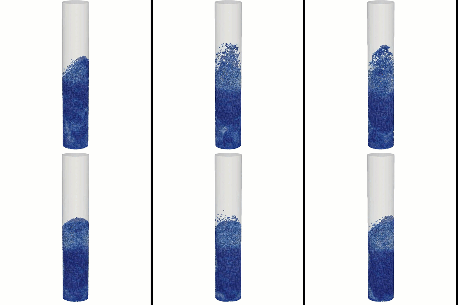
Introducing the tensorFB-DEM Fluidized Bed Template
The tensorFB-DEM template is a specialized configuration designed specifically for simulating gas–solid fluidized beds using a coupled 4-way CFD–DEM approach. Instead of treating the particles as a heavy, continuous fluid phase or forcing a brute-force calculation, this template couples a Eulerian fluid solver (OpenFOAM cfdemSolverPiso) with a discrete Lagrangian particle physics engine (LIGGGHTS). This methodology tracks the individual trajectories, rotations, and collisions of tens of thousands of unique spheres while simultaneously capturing the fluid drag and void-fraction fluctuations. If you use this specific template for your work, all that is asked is that you mention and give credit to tensorFB-DEM in your reports or projects.
How the Fluid and Particles are Arranged
The template sets up a classic cylindrical fluidization column measuring roughly 27.6 mm in diameter and 150 mm in height. The system initializes by packing and settling approximately 32,000 spherical particles with a 1 mm diameter and a density of 2000 kg/m³ at the bottom of the bed. For the gas phase, a specialized demo fluid enters through the bottom inlet nozzle, ramping its velocity from 0.02 to 0.15 m/s over a span of 0.2 seconds to exceed the minimum fluidization velocity. As the gas flows upward against gravity, the software automatically tracks the intense momentum exchange, drag history, and shifting void fractions across the bed.
How to Run Your First Simulation
Running the simulation inside the verified cfdem:local Docker container is handled through four simple script commands. First, you run a mesh pipeline command (blockMesh) to generate a high-resolution, multi-block fluid grid mapping the cylindrical column. Second, you launch a particle script (./parDEMrun.sh) to generate, pack, and settle the spheres into a steady baseline restart file. Third, you execute the master coupled solver script (./parCFDDEMrun.sh) to split the mathematical computation across 8 parallel MPI processors and compute the 2.0-second fluidization window. Finally, a cleanup script (./Allclean.sh) is available to instantly wipe away old runtime fields, logs, and particle dumps whenever you want a fresh start.
Adjusting Operating Conditions and Knobs
Changing your basic operational settings is incredibly straightforward and highly flexible. To modify fluid behavior, you can adjust the initial velocity profile, density, or kinematic viscosity files directly inside the CFD initial fields and transport properties dictionary. To adjust the solid phase, you can open the LIGGGHTS initialization script to scale the total particle count or modify the Hertzian contact mechanics properties—such as Young’s modulus and friction coefficients. The coupling interval frequencies can also be tuned directly within a centralized coupling properties dictionary to balance calculation speed with interfacial accuracy.
Post-Processing and Viewing Results
To visualize the coupled data, you run a post-processing script (./Allpostprocess.sh) that safely reconstructs the split fluid processor folders and converts the raw particle data into XML-compliant .vtp and .pvd time-series files. You can open the reconstructed fluid fields directly in ParaView using a .foam file placeholder to color the gas phase by local void fraction or velocity. Simultaneously, you can import the particle time-series to display the spheres using a Point Gaussian representation or a Sphere Glyph filter scaled precisely by the physical particle radius attribute.
A Quick Warning
Please keep in mind that this template is a development version utilizing optimized demo fluid properties and a soft Young’s modulus to ensure the case remains small, fast, and stable on standard computing setups. The accuracy of your final engineering answers depends entirely on your specific boundary conditions, grid resolution, and particle interactions, so pt-tensor.com does not take responsibility for the final simulation data. Always double-check your engineering results against physical validation data.
Author: Caesar Wiratama
Find me on Linkedin