
The definition of Boundary Conditions (BCs) in the CFD simulation plays a major role in the accuracy and reliability of the solution. There are lots of BC options that often overwhelm the user when choosing the right one. Even some commercial CFD solvers do not describe the mathematical details about it.
As a general reference, in this chapter, we will briefly describe the general rule of how the BCs are described so you can select it rigorously for your simulation.
6.1. Dirichlet and Neumann Condition
In fluid dynamics, we often face some conditions in which we can assume the value is constant on a specified plane, and sometimes, we face the condition that the gradient of a value is constant instead.
- Dirichlet Condition: or fixed value condition specified the boundary condition with a specified value, for example, constant temperature 300 K on a surface.
- Neumann Condition: or fixed gradient condition specified the boundary condition with the specified value of gradient in the normal direction
6.2. Wall Boundaries
Specifying mesh or cells as “wall” defines the normal velocity to that surface will be zero or non-penetrating.
The commonly used velocity boundary condition for the wall is a no-slip condition, which specifies the zero velocity on the wall.
This is true from the experimental observation that the velocity will approach zero toward the wall due to friction (viscosity 0). Or the velocity can be specified. If the wall is moving with a specified velocity, the fluid will “stick” to that velocity near the wall.
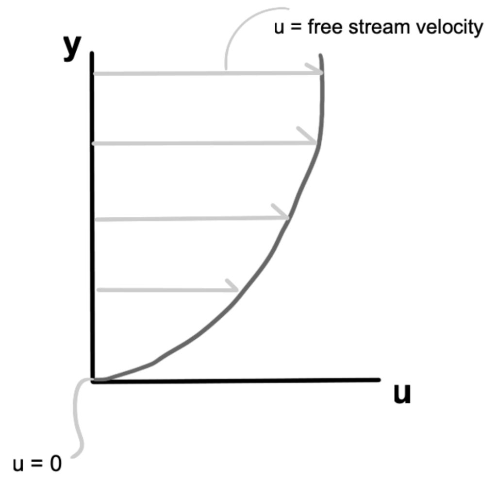
Figure 6.1. The Boundary Layer near the wall
The other option is the slip condition, which specifies the velocity value the same as the nearby velocity field. This is typically used to avoid the boundary layer effect near the object or represent the symmetry plane.
6.3. Ground Boundary for Vehicle
In external aerodynamics simulations of ground vehicles (cars, trucks, trains, or racing vehicles), the treatment of the ground boundary has a significant impact on the predicted aerodynamic forces, especially drag and lift.
If the ground is modeled as a stationary wall, a strong boundary layer develops along the ground surface. This boundary layer artificially thickens the near-ground flow and may lead to an over-prediction of drag and incorrect pressure distribution beneath the vehicle.
To better represent real driving conditions, a moving ground boundary condition is commonly applied. In this approach, the ground is modeled as a wall moving at the same velocity as the freestream (vehicle speed), typically in the opposite direction of the vehicle’s reference frame. Mathematically, this corresponds to a Dirichlet condition for tangential velocity, while maintaining a non-penetration condition in the normal direction.
Key characteristics of the moving ground condition are:
Zero normal velocity (no penetration).
Tangential velocity equal to the freestream velocity.
Elimination of the artificial ground boundary layer relative to the vehicle.
This approach mimics the relative motion between the vehicle and the road and is essential for accurate prediction of:
- Underbody flow behavior
- Ground effect and lift
- Diffuser and splitter performance
For high-fidelity automotive CFD simulations, the moving ground condition is often combined with rotating wheels, ensuring consistent relative motion between the wheels, ground, and incoming flow.
6.4. Inlets and Outlets
A disturbance in a flow is a change in the equilibrium of a fluid state, and this disturbance travels or propagates through the fluid via advection. Hence, it travels at the speed of sound.
The pressure equation describes wave propagation; a disturbance at any point simultaneously influences the solution everywhere. Then, pressure is the variable to be specified in the BC to support wave propagation.
Therefore, pressure is prescribed at the outlet as a Dirichlet BC, and for the inlet, we usually set the zero gradient of the pressure instead.
For velocity (or in the form of flow rate), the inlet condition is “physically” logical to set with the fixed value due to the fact that the disturbance propagates in the flow direction.
Another scenario is that we can define the pressure on the inlet and then set the zero gradient for the velocity; thus, the velocity will be calculated from the simulation. We cannot define both velocity and pressure simultaneously on the inlet.
For supersonic conditions (and compressible flow), waves can no longer propagate outwards the inlet BC. In this situation, a fixed value of pressure must be specified at the inlet. This is also true for the outlet; the normal pressure gradient should be applied instead.
6.5. Free (Entrainment)
In some cases, a single boundary mesh must act as both inflow and outflow; then, a BC for pressure and velocity can be defined as constant pressure (out pressure) and zero gradient velocity, but it is generally not recommended because it tends to make oscillating solution within the boundary, which leads to a divergent solution.
To accommodate the above problem, the total pressure BC can be used instead. For outflow, the pressure equals total pressure, but for the inflow, the pressure equals total pressure minus the dynamic pressure (represents the velocity).
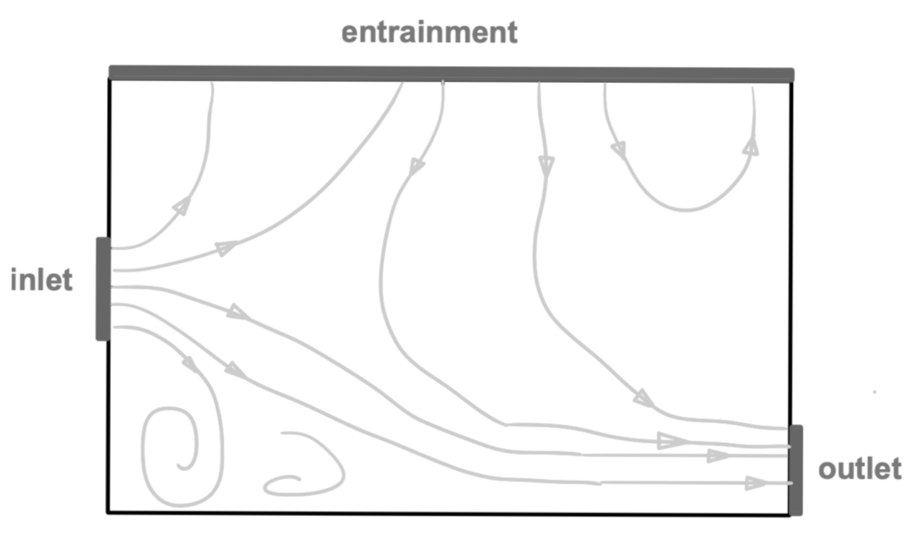
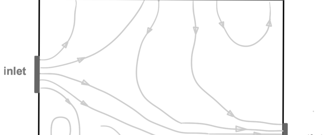
Figure 6.2. Entrainment Boundary Condition
6.6. Periodic Condition
As explained in Chapter 3, the required skill by CFD engineers is to simplify the problem without sacrificing accuracy and important physical phenomena. One useful way to do that is by utilizing periodic BCs.
6.6.1. Symmetry
This is a slip wall boundary, preventing flow from penetrating the plane. The tangential velocity on the symmetry plane is the same as the nearby stream velocity. Figure 3.1 illustrates the symmetry boundary condition.
6.6.2. Axisymmetry
Axisymmetry flow often occurs in engineering applications, such as flow in pipes, nozzle-diffuser, or injector spreading flow, and this can be reduced into a 2D domain while considering the “3D” rotating axis. The axisymmetry condition is illustrated in Figure 3.4.
6.6.3. Linear Periodic
Flow such as heat exchanger tubes, which involve a large amount of repetition, can be challenging to mesh. If the repetition is linear, this can be handled by using linear periodic.
The “outflow” of one periodic domain is used as the “inflow” of the other periodic domain, creating a realistic interaction and calculation within the domain.
It is important to note that in periodic conditions, the mesh of the paired periodic domain must be identical, which is often challenging.
6.6.4. Rotation Periodic
The flow of rotational periodic is often faced in engineering applications, such as wind turbine blades, propellers, fans, or maybe annular combustion chambers.
This basically works the same as linear periodic, but the domain is divided into a specified angles; for example, a wind turbines with 3 blades often constructed with 120-degree periodic domain.
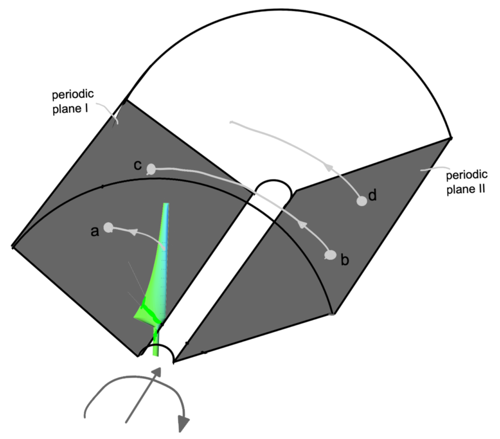
Figure 6.3. Rotation periodic boundary condition
From Figure 5.3 above, the turbine’s wake flow first reaches point “a” on the periodic plane I, then appears at point “b” on the periodic plane II, and so on until it reaches the outlet.
If we rotate this domain 120 two times to construct a full domain, the pattern will mimic the fully rotated flow. To make a periodic rotating flow, it is important to make sure the geometry and mesh of periodic planes are the same.
Modern post-processing software such as paraView can easily transform this periodic domain to visualize a “full” flow domain.
6.7. Multiphase boundary conditions
Multiphase flows involve the interaction of two or more phases, such as gas–liquid, liquid–solid, or gas–solid systems. In addition to the conventional flow variables (velocity and pressure), phase-specific variables—such as volume fraction, phase mass fraction, or interfacial properties—must also be prescribed at the boundaries.
At inlets, multiphase boundary conditions typically require:
- Fixed velocity or mass flow rate for the mixture or individual phases.
- Specification of phase volume fraction (e.g., liquid volume fraction α = 0.3).
- Optional phase-specific temperatures or properties if thermal effects are considered.
At outlets, a pressure outlet is commonly applied, with zero-gradient conditions for phase fractions. This allows the solver to naturally determine which phase leaves the domain, minimizing numerical reflections.
At walls, multiphase boundary conditions may include:
- No-slip or slip velocity conditions.
- Wall adhesion or contact angle models (important for liquid films, droplets, and wetting behavior).
- Phase-specific wall interactions such as deposition or rebound in particle-laden flows.
Improper specification of multiphase boundary conditions often leads to numerical instability, unphysical phase accumulation, or incorrect interface behavior. Therefore, consistency between inlet, outlet, and wall conditions is critical for maintaining mass conservation of each phase and achieving a stable solution.
6.8. Chemical boundary conditions
In reacting flow simulations, additional transport equations are solved for chemical species, and boundary conditions must be defined accordingly. These are referred to as chemical boundary conditions, which govern species mass fractions, reaction rates, and species fluxes at domain boundaries.
At inlets, chemical boundary conditions usually involve:
- Fixed mass fraction or mole fraction of each species (Dirichlet condition).
- Fixed temperature and velocity consistent with the chemical composition.
- In some cases, total mixture composition with individual species reconstructed internally by the solver.
At outlets, zero-gradient (Neumann) conditions for species mass fractions are commonly applied, allowing chemical products to exit the domain naturally without artificial constraints.
At walls, chemical boundary conditions can be classified into:
- Inert walls, where no species flux occurs (zero normal gradient).
- Reactive or catalytic walls, where species are consumed or generated according to specified surface reaction mechanisms.
- Deposition or ablation walls, where species mass flux is coupled with material removal or growth.
Correct chemical boundary condition selection is essential in simulations involving combustion, catalysis, corrosion, and chemical reactors. Inconsistent or over-constrained chemical BCs can easily lead to non-physical species accumulation or violation of mass conservation.
Author: Caesar Wiratama
Find me on Linkedin