
The computation process in CFD simulation is often constrained by hardware limitations due to huge mesh or small timesteps.
It becomes a mandatory skill for a good simulation engineer to reduce the model without sacrificing the important flow features needed to be simulated. Following are some model reductions by reducing the computational domain and mesh.
4.1. Symmetry domain
In some engineering applications, we often face a problem with a symmetrical nature, such as flow over a cylinder, road vehicle, or even aircraft, as long as the flow direction is parallel to the object direction, with no sideslip angle.
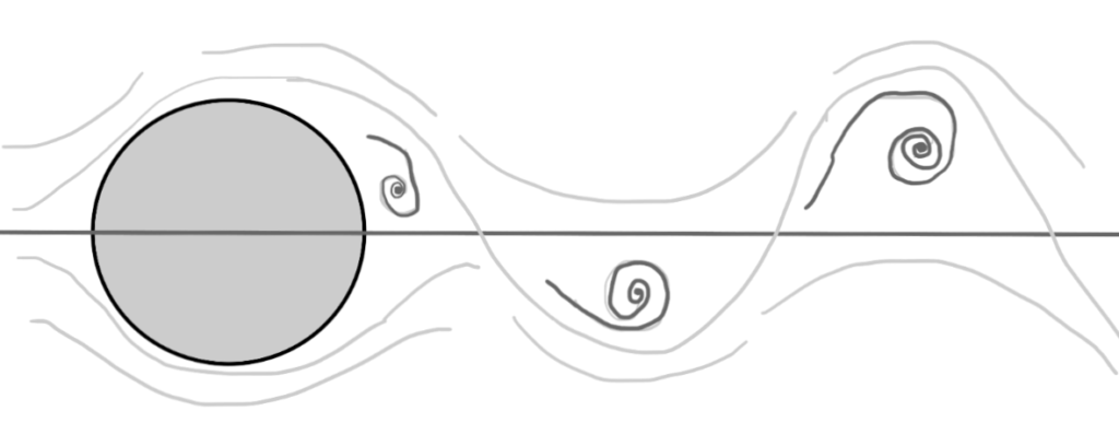
Figure 4.1. Parallel flow (top) and flow with sideslip angle (bottom)
Please note that even if the geometry is symmetrical in transient cases, it sometimes involves unsymmetrical flow behavior, such as a vortex shedding over a cylinder.
Figure 4.2. Vortex shedding over a cylinder
If the problem is symmetry, the domain can simply be divided into two, which, in the end, reduces the total mesh in half and makes the computational effort much less.
The symmetry boundary condition basically has behavior similar to slip plane wall, which is a transform condition, so for the scalar variable, the gradient will be zero, and for the vector, the gradient in the tangential direction will be zero and has zero value normal to the plane.
4.2. Periodic flow
Often encountered in fluid flow modeling, scenarios like heat exchangers with a large number of tubes can render the geometry too complex for modeling and simulation. This complexity demands high computational effort (hardware specifications, expertise, time, etc.), making it infeasible.
If the flow features are repetitive or periodic, such as tubes in a heat exchanger, periodic flow modeling within CFD can be employed.
Generally, periodic flow is divided into two types: (1) streamwise-periodic or fully developed periodic, which entails a repeating pattern aligned with the flow generating a pressure drop, and (2) periodic patterns perpendicular to the flow, not causing any pressure drop along their repeating direction.

Figure 4.3. Periodic flow
4.3. Swirling and rotating flow
In general engineering applications, swirling flows are quite common, such as the fuel-air mixing in a combustion chamber, mixing tanks, and so forth.
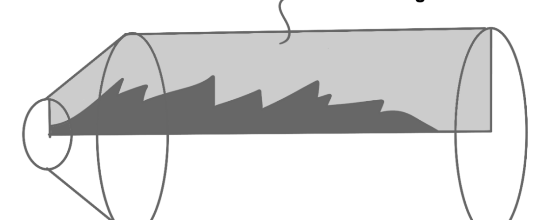
CFD modeling also enables the simulation of such flows with a 2D simplification, given that the flow exhibits axisymmetry (symmetry around a particular rotational axis), as illustrated in Example Figure 3.4 below:
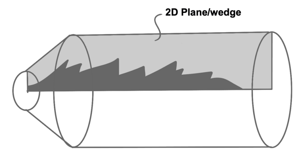
Figure 4.4. Combustion chamber axisymmetry modeling
Following is the momentum equation for 2D swirling flow in general:
(3.1)
For flows with pressure gradients in the circumferential direction, a 2D modeling approach is not feasible.
However, no specific procedure is needed to create a 3D swirling flow model, but the computational effort will much larger.
4.4. Moving reference
In many system analysis applications, systems often require unsteady analysis, such as the rotation of turbine rotors or pumps.
To simplify this analysis into a steady-state analysis, making it easier to set up and reduce computational effort, in CFD, we can “move” the system’s coordinate system without actually shifting the system concerning its inertial coordinate system.
This modeling approach is known as the moving reference frame. This method can impart translational or rotational motion to a system.
For example, we can rotate the entire domain in cases like wind turbines or rotating propellers without affecting surrounding parts. This analysis is also known as the single reference frame (SRF). The simplification of impeller rotation in the SRF case is illustrated in Figure 3.5 below:
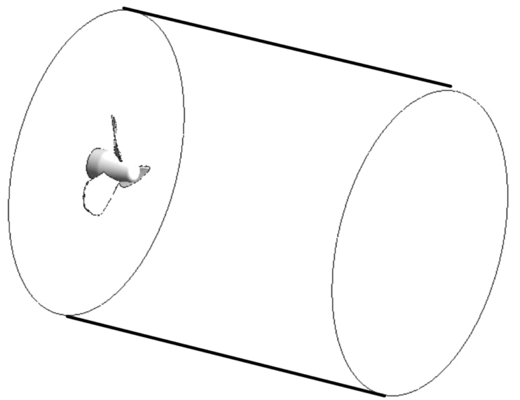
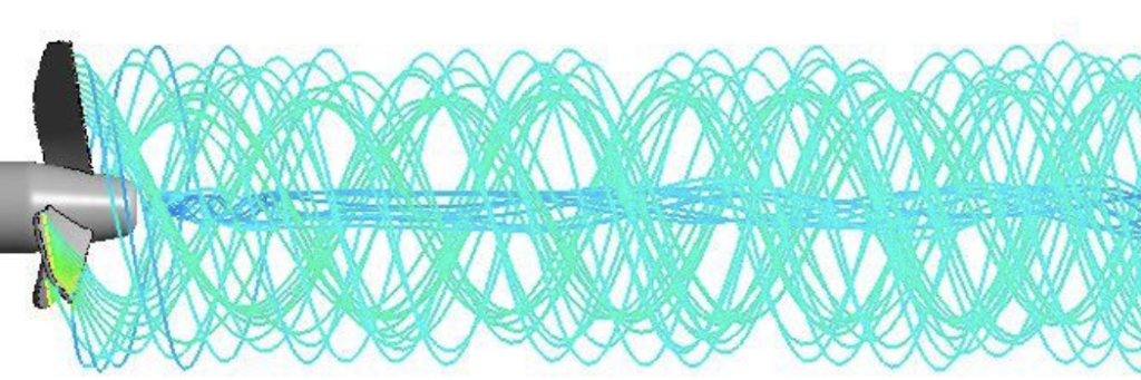
Figure 4.5. Single Reference Frame (SRF) domain (top) and simulation result (bottom) of a propeller
However, we need to rotate the domain without moving the surrounding area for gas turbines or pumps with a stator or volute surrounding them. In other words, this system has multiple reference frames (MRF). This is illustrated in Figure 2.15 in the previous chapter.
Although the idea behind engineering a moving reference frame is to transform the unsteady analysis of a system, viewed from the stationary (inertial) coordinate system, into a steady one in the moving coordinate system, we can still conduct unsteady analysis as well.
For instance, in the analysis of vortex shedding – an unsteady phenomenon resulting from flow instability – it produces unsteady flow, not due to the unsteady effect of the rotation of the inertial coordinate system.
4.4.1. Moving reference frame equation
Let’s say we have a coordinate system that translates with a linear velocity and rotates with an angular velocity
relative to the inertial coordinate reference, as illustrated in the image below:
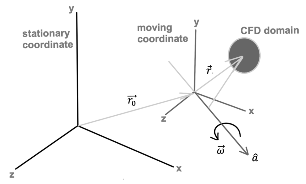
Figure 4.6. Moving coordinate system
The center point of the coordinate system is represented using a position vector, .
The center of rotation defined with vector , hence
.
The computational domain for solving CFD solutions is defined with respect to a moving reference system, so a point within the CFD domain is located at position vector from the center of the moving coordinate system.
Then, the flow velocity can be transformed from the inertial coordinate system to the moving coordinate system using the equation , where
.
In the above equation, is a relative velocity (velocity observed from moving coordinate),
is the absolute velocity (velocity observed from inertial coordinate),
is the velocity from moving reference relative to inertial ,
is translational velocity, and
is rotational velocity.
When solving the motion equations in the moving coordinate system, the fluid acceleration will have additional terms that arise from the momentum equation.
This can be formulated in two ways: (1) using the relative velocity formulation by expanding the momentum equation with relative velocity as the dependent variable, and (2) using the absolute velocity formulation by expanding the momentum equation using absolute velocity as the dependent variable.
Equation (3.2) represents the momentum equation in the relative velocity formulation, while equation (3.3) represents the momentum equation for the absolute velocity formulation.
(4.2)
Where, .
(4.3)
In equation (3.2) the also known as Coriolis acceleration, and
is centripetal acceleration.
And in equation (3.3) Centripetal and Coriolis acceleration can be modified to .
4.4.2. Multiple Reference Frames Equation (MRF)
In multiple reference frame modeling, there are typically two or more domains, one of which is a moving domain while the others are stationary.
This case is commonly found in situations involving rotating objects with a nearby stator, such as gas turbines, blowers with volutes, or mixing tanks with baffles.
The example case of MRF with one static domain and more than one rotating domain is the simulation of a multirotor using four propellers. One static domain is the fluid domain around the airframe, and the four rotating domains are each propeller, each having its independent moving coordinate system.
Author: Caesar Wiratama
Find me on Linkedin