
Computational Fluid Dynamics, or CFD, is relatively new compared to the development of fluid mechanics theory itself. Basically, CFD is a method of numerical analysis that analyzes and solves fluid dynamics problems.
The equation of fluid mechanics actually can be solved using general physics law, such as conservation of mechanical energy, Newton’s law, or conservation of mass; but, unfortunately, the nature of the equation involving complex tensor nonlinear partial differential equations which cannot be solved analytically (except you make the 1D, incompressible, inviscid assumption: which is often not the chase for the real world application.
Due to this mathematical complexity, the numerical method has become the best choice (so far) to make the fluid dynamic equation useful for our real-world application, which makes the CFD program quite popular.
The trend of cost of computation (hardware and software) has also become much more conducive than when the CFD was developed.
INDUSTRIAL UTILIZATION OF CFD
Because CFD solves general fluid dynamic equations (Navier-Stokes equation, or sometimes Lattice Boltzmann), it allows this program to solve complex turbulent, viscous, compressible, heat transfer, and much more; hence, the applications are also varied, ranging from aerospace, automotive, maritime, chemical process, energy generation, civil engineering, urban planning, electronics, consumer goods, bioengineering, and more.
Using a numerical model that can be solved by a computer, we can obtain extremely valuable information, such as velocity, pressure, or temperature at any specific point and time for even a complex geometry. This allows engineers to better understand the detailed physical phenomena and make a precise design judgment.
Without any physical fabrication and laboratory, an organization can save a huge amount of money. Moreover, the absence of physical experiments eliminates the risk of testing failure, which is extremely useful for extreme scenarios such as high-speed rotation, combustion, or explosion tests.
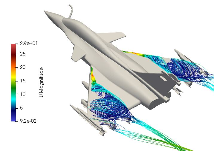
Figure 1.1. Simulation of the rolled-up vortex on a delta wing aircraft (OpenFOAM)
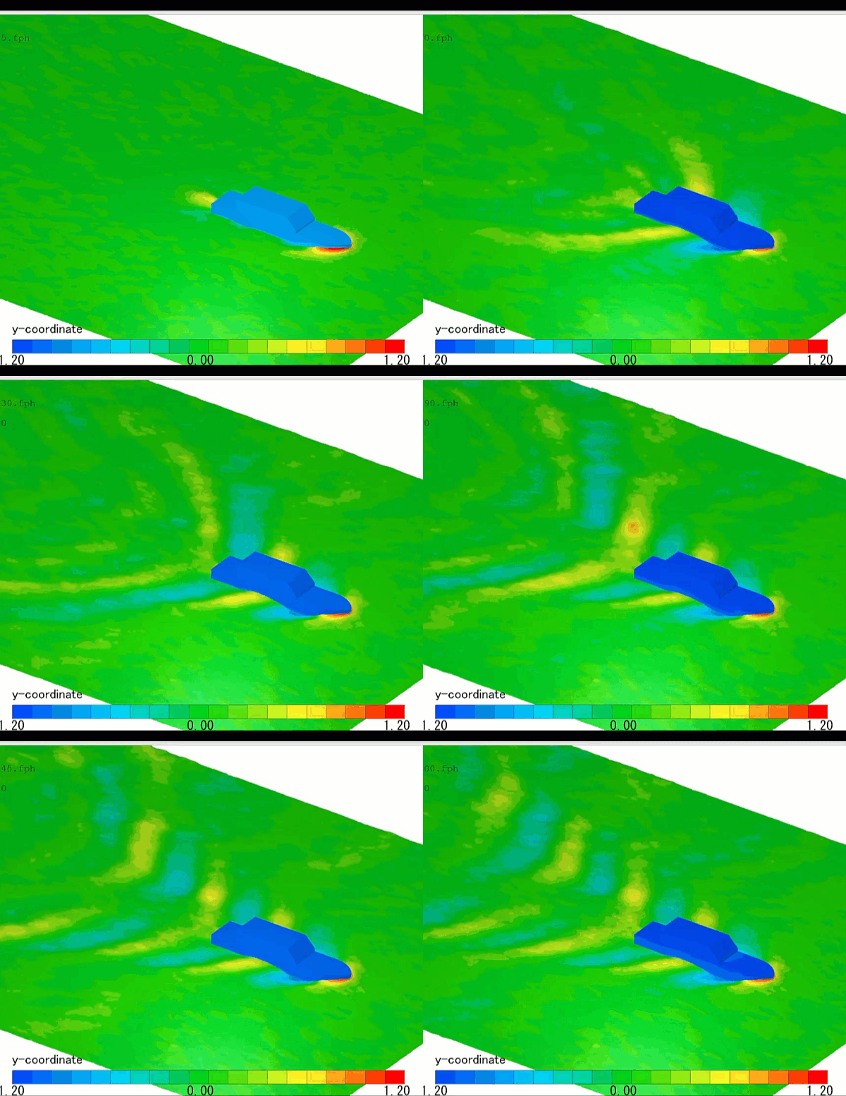
Figure 1.3. Simulation of a wave generating drag over a hull (Cradle CFD)
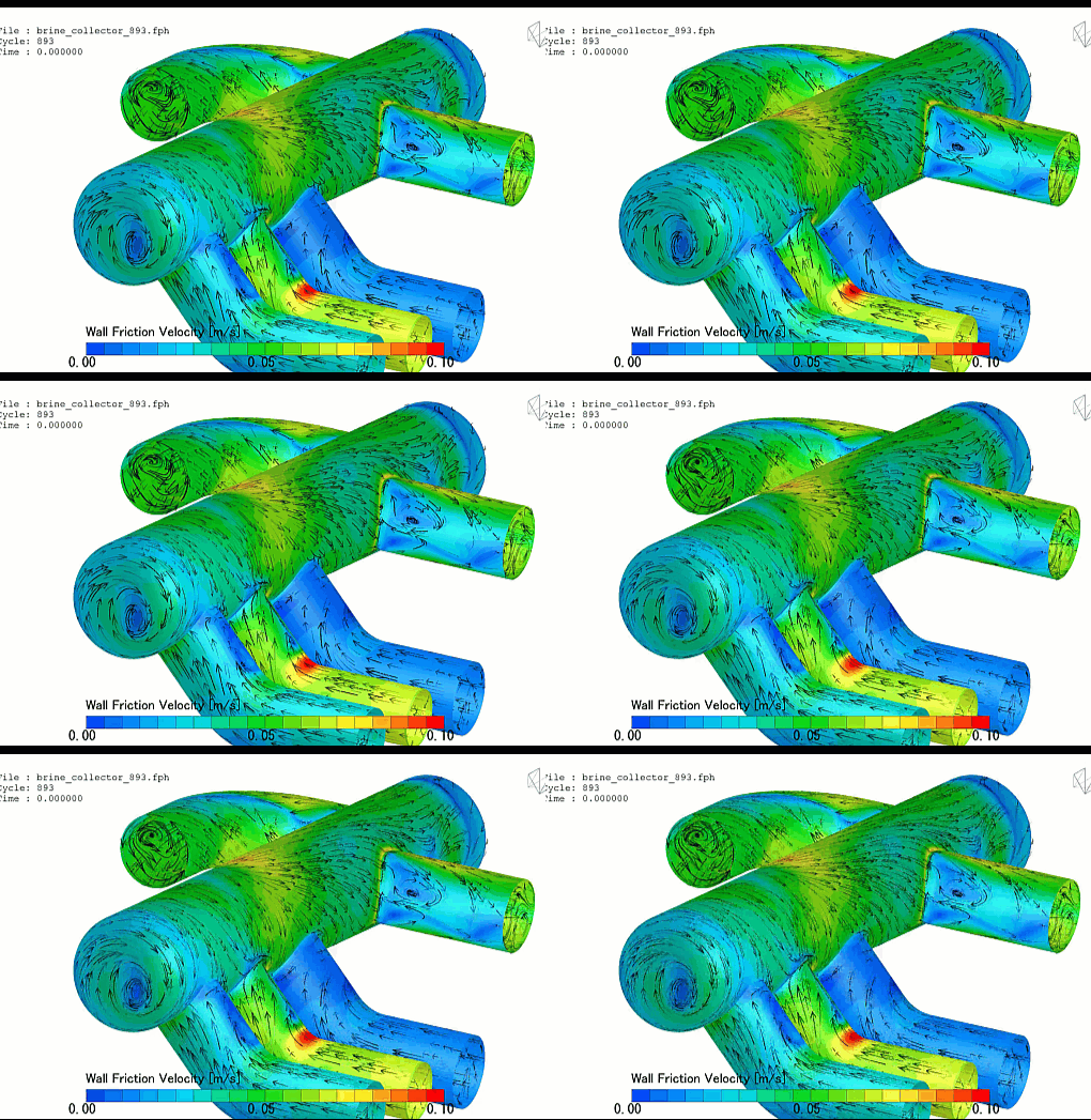
Figure 1.4. Simulation of flow within the chemical process piping (Cradle CFD)
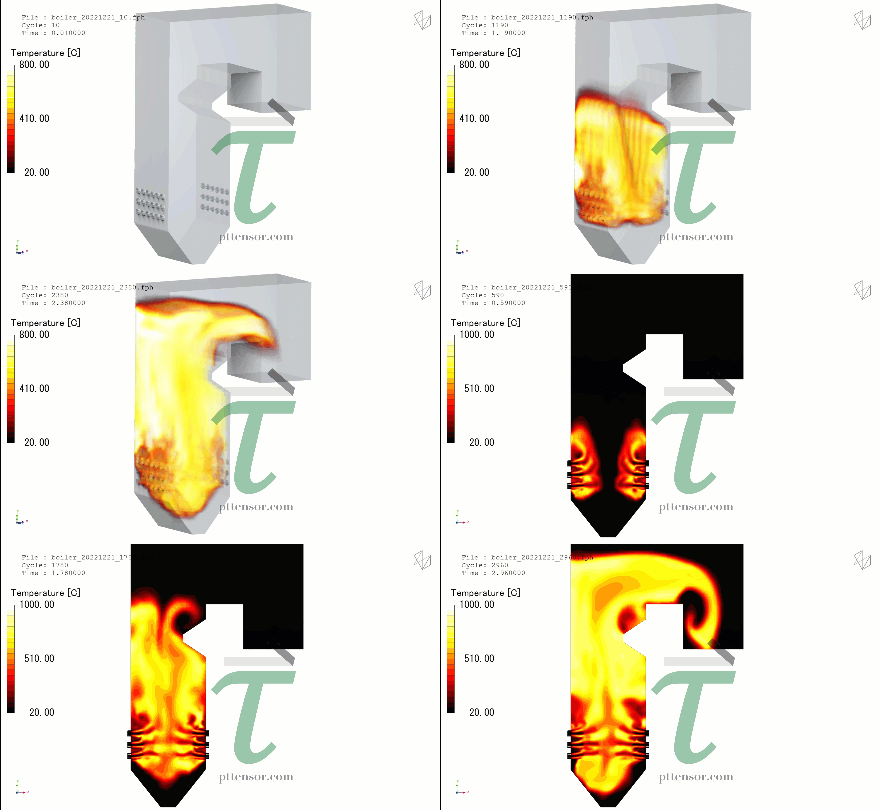
Figure 1.5. Simulation of combustion in the coal-fired boiler (Cradle CFD)
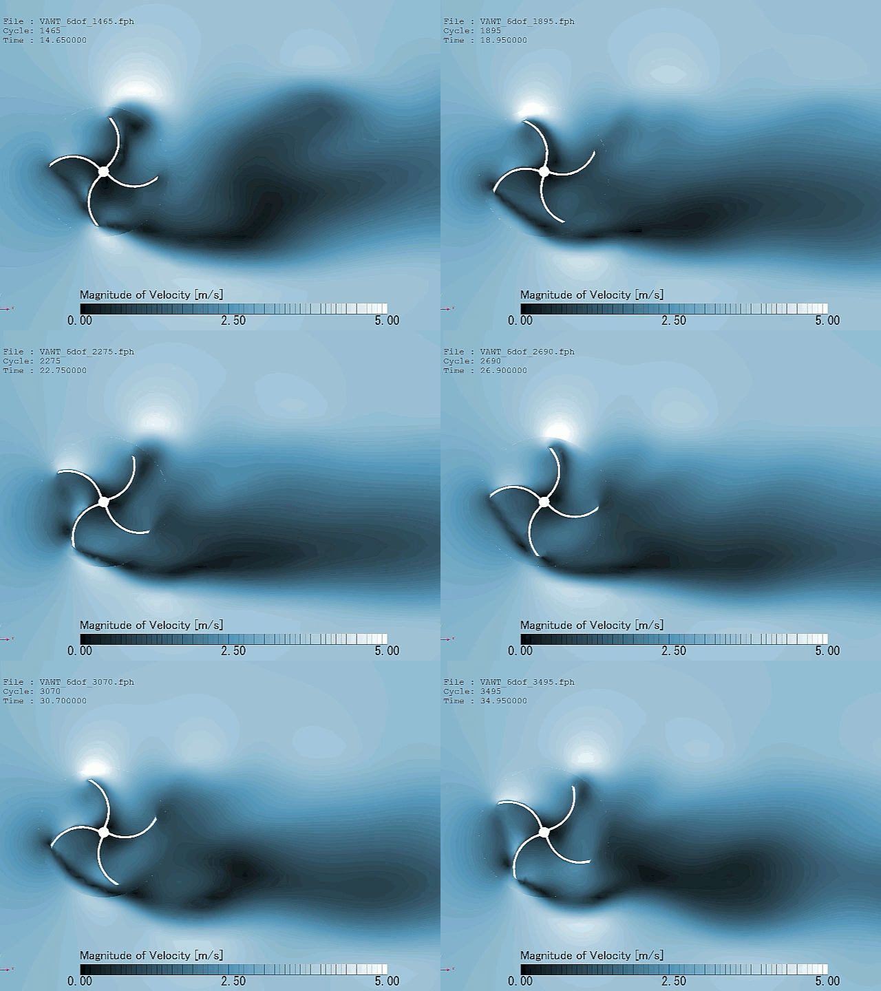
Figure 1.6. Simulation of Vertical Axis Wind Turbine (Cradle CFD)
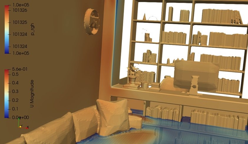
Figure 1.7. Simulation of HVAC In a Building (tensorHVAC-Pro)
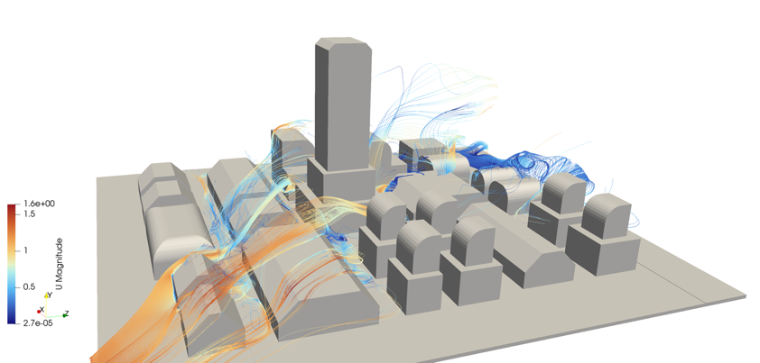
Figure 1.8. Simulation of wind around the building for urban planning (tensorHVAC-Pro)
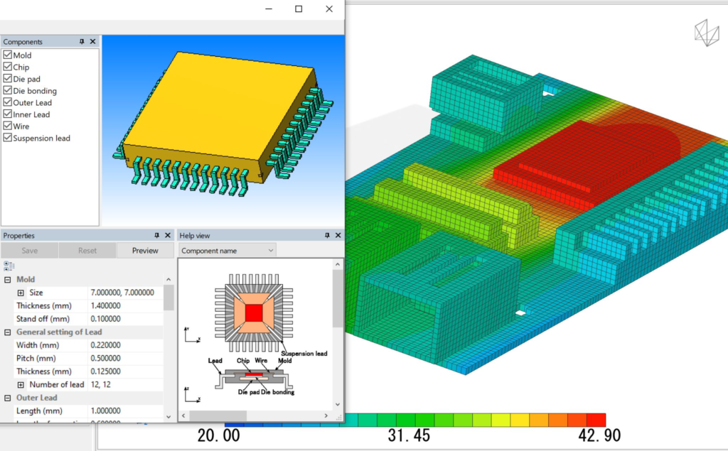
Figure 1.9. Analysis of PCB heating (Cradle CFD)
HISTORY OF CFD
Generally, the fundamental problem of CFD is solving the Navier-Stokes equations. Historically, the first method developed was 2D flow around an airfoil using conformal transformation, which was developed in the 1930s.
Lewis Fry Richardson used the idea of calculating using finite differences. In 1922, he divided the physical space into cells in the book Weather Prediction by Numerical Process, although the prediction was not entirely satisfactory.
From 1957 to the late 1960s, a group at Los Alamos National Lab, the T3 group led by Francis H. Harlow, developed three-dimensional methods such as particle-in-cell, fluid-in-cell, vorticity stream function, and marker-and-cell methods.
The first paper with a three-dimensional model was published in 1967 by John Hess and A.M.O. Smith of Douglas Aircraft. Panel methods are a method of discretizing the surface of the geometry with panels. The lifting panel code (A230) was described in a paper by Paul Rubbert and Gary Saaris in Boeing 1968. From this, more advanced methods were developed to be used in the development of submarines, surface ships, automobiles, helicopters, aircraft, and wind turbines.
In the early 1980s, Richard Eppler developed the PROFILE code, partly with NASA funding. This code performs 2D airfoil analysis with boundary layer analysis, including viscous effects. Mark Drela’s XFOIL code soon followed it.
Also, in the early 1980s, an intermediate step between Panel and full potential codes was used to transonic small disturbance equations, the 3D WIBCO code, developed by Charlie Boppe of Grumman aircraft.
Developers turned to Full potential codes because the Panel method could not calculate non-linear flow at transonic speeds. Frances Bauer, Paul Garabedian, and David Korn from New York University (NYU) wrote a series of 2D full potential airfoil codes that were widely used, the most important being Program H. Antony Jameson, also from NYU, worked with David Caughey to develop the important 3D Full potential code FLO22 in 1975. Many full potential codes emerged after this, culminating in Boeing’s Tranair (A633) code.
In 1981, Jameson developed the 3D FLO57 code from Lockheed’s TEAM program based on the Euler equation. The program uses structured cartesian mesh code, while most others use structured body-fitted grids.
Recent CFD codes can solve granular materials using chemical processes and physical models.
GENERAL WORKFLOW OF CFD
Generally (simplified), the steps involved in the CFD process are summarized in the flowchart below:
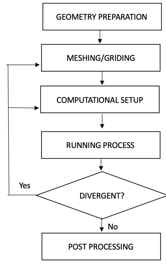
Figure 1.11. General (simplified) CFD workflow
In common modern CFD packages, the geometry can be easily imported from Computer-Aided Design (CAD) software, such as Solidworks, Autodesk Inventor/Fusion 360, Catia, or an open-source modeler such as Blender with various extensions depending on the software’s compatibility.
For more traditional CFD packages, in some cases that need high-quality mesh, the geometry is sometimes constructed manually while creating the mesh, ensuring the consistency of the mesh structure. This is sometimes only limited to simple and primitive geometries such as blocks or spheres.
The next step is meshing/griding, a process of converting continuous geometry (1D/2D/3D) into discrete form, in which we solve the equation within each discrete element. This process can be done automatically or manually, depending on the software package; sometimes, we use a different software package or brand only for meshing and then import it to the solver with the other package/brand.
After the mesh is set up, the following process is to solve the discrete equations inside each discrete mesh element, which stores the resulting data such as velocity, pressure, temperature, etc. Each software package sometimes has different capabilities and limitations for the solver; for example, some solvers can only solve incompressible flow or have no heat transfer. So, engineers should carefully read the solver they are using based on the physical phenomena they are facing.
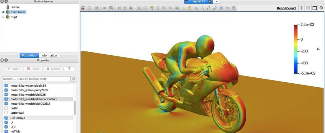
To interpret the result, the solution can be plotted as curves or 3D-colored contours. This process is called post-processing. Again, some software sometimes uses a different package/brand to do the post-processing. Or, a popular open-source post-processing tool such as paraView can sometimes be used for various extensions.
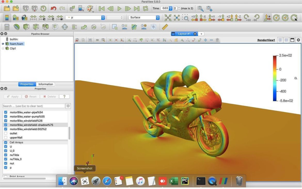
Figure 1.12. Post-Processing using ParaView
Author: Caesar Wiratama
Find me on Linkedin